Bias Neurons using R

The concept of bias in neural networks is fundamental to their ability to model complex relationships and perform various tasks, including classification, regression, and deep learning. In this theory overview, we’ll explore what bias neurons are, why they are essential, and how they work in the context of neural networks.

What is a Bias Neuron?

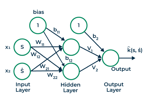
A bias neuron (or bias unit) is a special neuron in a neural network that does not have any inputs but is always connected to the other neurons in a layer. It serves as a learnable parameter in the network, allowing each neuron to learn an offset or shift in its activation function. In R Programming Language This offset helps the network fit the data more accurately and increases its expressive power.

Bias Neurons using r

Purpose of Bias Neurons

• Handling Non-Zero Intercept: Without bias neurons, the neural network can only model functions that pass through the origin (0,0) of the input space. However, many real-world problems require models that don’t necessarily go through the origin. Bias neurons allow neural networks to approximate functions with non-zero intercepts.
• Learning Offsets: In a neural network, the input data is linearly combined with weights, and the result is passed through an activation function. Without bias terms, the network can only learn the shape and orientation of functions. Bias terms enable the network to learn vertical shifts in the activation function, which is crucial for fitting data that isn’t centered around zero.
• Expressive Power: Including bias terms increases the expressive power of the neural network. It allows the network to represent a wider range of functions and capture more complex relationships in the data.
• Overcoming Symmetry: Bias neurons break the symmetry that exists when all neurons in a layer have identical inputs and weights. Symmetry can lead to difficulties during training and hinder convergence. Bias terms help to overcome this issue.

Role in Neural Network Layers

Bias neurons are usually included in each layer of a neural network. In a typical feedforward neural network, they have no inputs but are connected to all neurons in the subsequent layer. Mathematically, they add a constant value to the weighted sum of inputs before applying the activation function. The bias term is adjusted during training through backpropagation, just like the weights.

Training Bias Neurons

During the training process of a neural network, the values of the bias neurons are updated alongside the weights using optimization algorithms like stochastic gradient descent (SGD). The goal is to minimize a loss function that quantifies the difference between the network’s predictions and the true target values. The optimization algorithm seeks to find the optimal bias values that minimize this loss.

Example for Bias Neurons using R

The Keras library that demonstrates the role of bias neurons in a neural network. In this example, we’ll create a single neuron (perceptron) with bias.

Generate sample data

R

# Generate sample data
set.seed(123)
# 10 random input values for x1 and x2
x1 <- runif(1000)
x2 <- runif(1000)
# Linear relationship with some noise
y <- 2 * x1 + 3 * x2 + 1 + rnorm(5, mean = 0, sd = 0.1)

We generate some sample data, x as input and y as the output, representing a linear relationship y = 2x + 1 with some random noise.

Create Model

R

# Load the required libraries
library(keras)

# Create a sequential model
model <- keras_model_sequential()

# Add a hidden layer with, for example, 2 units and ReLU activation
model %>%
  layer_dense(units = 2, activation = 'relu', input_shape = c(2), use_bias = TRUE)

# Add the output layer with 1 unit (for regression) and linear activation
model %>%
  layer_dense(units = 1, activation = 'linear',use_bias = TRUE)  # For regression

# Compile the model with a loss function, optimizer, and metric (e.g., mean squared error for regression)
model %>% compile(
  loss = 'mean_squared_error',  # You can change the loss function based on your problem
  optimizer = 'adam',
  metrics = c('mean_absolute_error')  # You can choose appropriate metrics
)

# Summary of the model
summary(model)

Output:

Model: "sequential_1"
________________________________________________________________________________
 Layer (type)                       Output Shape                    Param #     
================================================================================
 dense_2 (Dense)                    (None, 2)                       6           
 dense_3 (Dense)                    (None, 1)                       3           
================================================================================
Total params: 9 (36.00 Byte)
Trainable params: 9 (36.00 Byte)
Non-trainable params: 0 (0.00 Byte)
________________________________________________________________________________

We create a sequential model and add a dense layer with one neuron using layer_dense. The use_bias = TRUE argument ensures that bias is included.

• We compile the model with the mean squared error loss function and the Adam optimizer.
• We train the model for 100 epochs using the sample data.
• Finally, we retrieve the learned weight and bias values using get_weights and print them.

Train the model

R

# Train the model
history <- model %>% fit(
  cbind(x1, x2), y,  # Use cbind to provide both x1 and x2 as input
  epochs = 500,
  verbose = 0
)

# Get the learned weights and bias
weights <- get_weights(model)
print(weights)

Output:

[[1]]
           [,1]      [,2]
[1,] -1.1044016 0.9812743
[2,] -0.5948815 1.4780935

[[2]]
[1] 0.0000000 0.3192987

[[3]]
          [,1]
[1,] 0.1048971
[2,] 2.0368812

[[4]]
[1] 0.2609277

Hidden Layer ( Or First Layer) weights and Bias

R

# Extract and print the learned weights and biases for the first hidden layer
hidden_layer_weights <- get_weights(model$layers[[1]])

w11 <- hidden_layer_weights[[1]][1]  # Weight from x1 to the 1st hidden unit
w21 <- hidden_layer_weights[[1]][2]  # Weight from x2 to the 1st hidden unit
w12 <- hidden_layer_weights[[1]][3]  # Weight from x1 to the 2nd hidden unit
w22 <- hidden_layer_weights[[1]][4]  # Weight from x2 to the 2nd hidden unit

b11 <- hidden_layer_weights[[2]][1]   # Bias for the 1st hidden unit
b12 <- hidden_layer_weights[[2]][2]   # Bias for the 2nd hidden unit

cat("Weight (x1 to 1st hidden unit): w11 =", w11, "\n")
cat("Weight (x2 to 1st hidden unit): w12 =", w12, "\n")
cat("Weight (x1 to 2nd hidden unit): w21 =", w21, "\n")
cat("Weight (x2 to 2nd hidden unit): w22 =", w22, "\n")
cat("Bias (1st hidden unit): b11 =", b11, "\n")
cat("Bias (2nd hidden unit): b12 =", b12, "\n")

Output:

Weight (x1 to 1st hidden unit): w11 = -1.104402 
Weight (x2 to 1st hidden unit): w12 = 0.9812743 
Weight (x1 to 2nd hidden unit): w21 = -0.5948815 
Weight (x2 to 2nd hidden unit): w22 = 1.478094 
Bias (1st hidden unit): b11 = 0 
Bias (2nd hidden unit): b12 = 0.3192987

Learned weights and bias for the output layer

R

# Extract and print the learned weights and bias for the output layer
output_layer_weights <- get_weights(model$layers[[2]])

v_1 <- output_layer_weights[[1]][1]  # Weight from H11 to the output
v_2 <- output_layer_weights[[1]][2]  # Weight from b12 to the output
b_2 <- output_layer_weights[[2]]  # Bias for the output layer

cat("Weight (H11 to the output): v1 =", v_1, "\n")
cat("Weight (H12 to the output): v2 =", v_2, "\n")
cat("Bias (for the output): b2 =", b_2, "\n")

Output:

Weight (H11 to the output): v1 = 0.1048971 
Weight (H12 to the output): v2 = 2.036881 
Bias (for the output): b2 = 0.2609277 

The printed values of “Learned Weight” and “Learned Bias” should be close to 2 and 1, respectively, indicating that the model has learned the linear relationship with bias. The bias term allows the model to capture the non-zero intercept of the linear function.

Plot the computation graph of the model

R

# Plot the computation graph of the model
plot(model,show_shapes = TRUE)

Output:

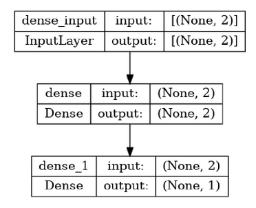
Simple 2 Layer Neural Network

We can plot the model using plot function and shows all the layers in owr model.

Predictions using Model

R

# Assuming you have already trained the model and obtained the 'model' object
x1 = 2
x2 = 3
# Create a data frame with the input values matching the model's input layer name
new_data <- cbind(x1, x2)

# Use the model to make predictions
predictions <- model %>% predict(new_data)

# Print the prediction
cat("Trained Model prediction for x1 = 2 and x2 = 3:", predictions, "\n")

x1 =2
x2 =3

h11 = (w11*x1+w21*x2+b11)
# Apply ReLU activation
h11_relu <- ifelse(h11 > 0, h11, 0)
h12 = (w12*x1+w22*x2+b12)
# Apply ReLU activation
h12_relu <- ifelse(h12 > 0, h12, 0)
cat('First hidden neuron value :',h11_relu,'\n')
cat('Second hidden neuron value :',h12_relu,'\n')

Output = h11_relu*v_1 + h12_relu*v_2 + b_2
cat('Model prediction using the Trained Weights & Biases for x1 = 2 and x2 = 3:',Output,'\n')

Output:

Trained Model prediction for x1 = 2 and x2 = 3: 13.94088 
First hidden neuron value : 0 
Second hidden neuron value : 6.716128 
Model prediction using the Trained Weights & Biases for x1 = 2 and x2 = 3: 13.94088

Conclusion

Bias neurons are essential components of neural networks, allowing them to handle non-zero intercepts, learn offsets, increase their expressive power, and break symmetry. They are trained alongside weights to make the network capable of modeling complex relationships in the data. Understanding the role of bias neurons is fundamental in building and training effective neural networks for various machine learning and deep learning tasks.