Basic signal operations are nothing but signal manipulation or modification tools that are used in signal processing and analysis. It helps to understand the signals in different situations. These operations allow the modification and enhancement of signals for specific applications.
In this article, we will discuss the basic signal operations and understand different operations related to the time and amplitude of the signal. In time transformations, we will cover time scaling, time shifting, and time reversal, and in amplitude transformations amplitude scaling of signals, amplitude reversal of signals, addition of signals, multiplication of signals, differentiation of signals and integration of signals. We also cover various advantages, disadvantages and applications of time and amplitude transformations.
What are Basic Signal Operations?
Basic Signal Operations refer as the fundamental operations that can be performed on signals. These operations are fundamental in analyzing and manipulating signals for various operations such as telecommunications, audio processing, image processing, and control systems. These operations can be modified with respect to time and amplitude characteristics. Next, we will classify the Basic Operation of Signals
Classification of Basic Operation on Signals
The operation of the Signal can be performed on two variable parameter
Basic Signal Operations Performed on Amplitude
Basic operations on dependent variable amplitude also known as amplitude transformations. In which we manipulate or modify the amplitude of the signal by applying mathematical operations to its amplitude while the time axis of the signal is constant.
These are six basic amplitude transformations, which are :
- Amplitude scaling of signals
- Amplitude reversal of signals
- Addition of signals
- multiplication of signals
- Differentiation of signals
- Integration of signals
Amplitude Scaling of Signals
Amplitude scaling is the amplification or attenuation of the signal. By using amplitude scaling, we can increase or decrease the strength or gain of the signal, which depends on the scaling factor.
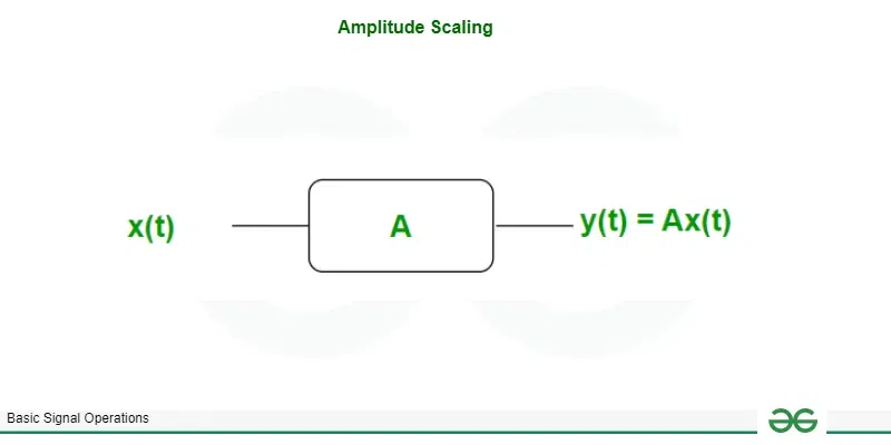
Block diagram of Amplitude scaling
The scaling factor is ‘ A ‘ then the amplitude scaled signal can be represented as Ax( t) where A is a positive value.
if A>1 ; signal is Amplified
0< A<1 ; signal is Attenuated
Example – A signal is x(t) shown below. find y1(t) = 2x(t) and y2(t) = 0.5x(t) ?

Given signal x(t)
x(t) = 1 ; [Tex]
-2 \leq t \leq 1[/Tex]
0 ; otherwise
y1(t) = 2x(t) ,
y1(t) = 2 ; [Tex]
-2 \leq t \leq 1[/Tex]
0 ; otherwise
y2(t) = 0.5x(t)
y2(t) = 0.5 ; [Tex]-2 \leq t \leq 1[/Tex]
0 ; otherwise
Graphically,
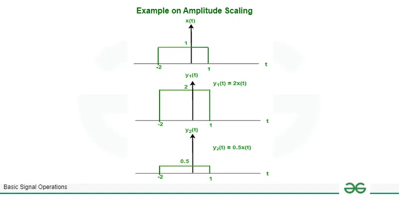
Amplitude scaling of signals
Amplitude Reversal of Signals
The amplitude reversal is the folding of the signal about the horizontal axis, or it is simply a mirror image about the horizontal axis. Amplitude reversal gives a 180-degree phase shift with respect to the horizontal axis.
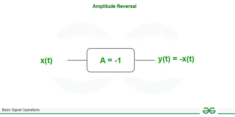
Block diagram of amplitude reversal
Example – let a signal is x(t) then find y(t) = -x(t)?
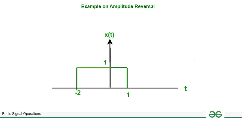
given signal x(t)
x(t) = 1 ; [Tex]
-2 \leq t \leq 1[/Tex]
0 ; otherwise
y(t) = -x(t) ,
y(t) = -1 ; [Tex]
-2 \leq t \leq 1[/Tex]
0 ; otherwise
Graphically ,

Amplitude reversal
Addition of Signals
The addition operation of two or more signals consists of adding amplitude of all the signal at every instant of time or space, resulting in new signals that have the characteristics of all signals combined together.
Mathematical representation of addition of signals
Let X1(t) , X2(t) , …………….. Xn(t) are n signals which are added to produce a new signal Y(t).
Then, Y(t) = X1(t) + X2(t) + X3(t)+ …………….. + Xn(t)
Example: Let X1(t) , X2(t) are two signals on which we have applied addition operation of signals that results y(t) then find the signal y(t)?

Given signals X1(t) and X2(t)
Solution:
X1(t) = 1 ; [Tex]-1 \leq t \leq 3[/Tex]
0 ; otherwise
X2(t) = 2 ; [Tex]0 \leq t \leq 2[/Tex]
0 ; otherwise
then y(t) = X1(t) + X2(t)
y(t) = 1 ; [Tex]-1 \leq t \leq 0[/Tex]
2 ; [Tex]0 \leq t \leq 2[/Tex]
1 ; [Tex]2 \leq t \leq3[/Tex]
0 ; otherwise
Graphically,
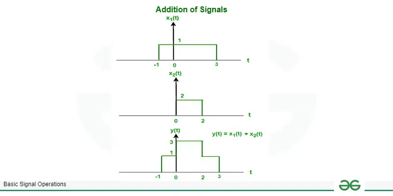
Solution of example on addition of solution
Multiplication of Signals
Signal multiplication is also a basic signal operation. The multiplication of two or more signals involves multiplying their amplitudes, which creates a new signal. This basic operation is very useful in the process of modulation, filtering etc.
Mathematical representation of multiplication of two signals:
Let X1(t) and X2(t) are two signals which are multiplied to create a new signal Y(t)
Then, Y(t) = X1(t) . X2(t)
Example: X1(t) and X2(t) are two signals shown below. Find Y(t) = X1(t) . X2(t) ?
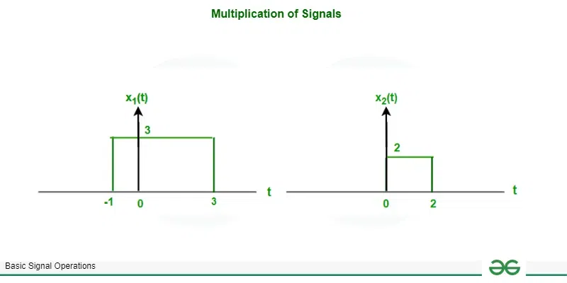
Given signals x1(t) and x2(t)
X1(t) = 3 ; [Tex]-1 \leq t \leq 3[/Tex]
0 ; otherwise
X2(t) = 2 ; [Tex]0 \leq t \leq2[/Tex]
0 ; otherwise
then Y(t) = X1(t) . X2(t)
Y(t) = 6 ; [Tex]0 \leq t \leq 2[/Tex]
0 ; otherwise
Graphically,

Solution of example on multiplication of signals
Differentiation of Signals
The operation of differentiation of signal is only applicable to continuous–time signals as differentiation is not defined for discontinuous signals. It represents instantaneous slope or the rate of change of the continuous signal with respect to time.
Mathematical representation of differentiation of signal:
Let x(t) is a continuous-time signal and y(t) represents differentiation of x(t)
then, [Tex]y(t) = \frac{d x(t)}{dt}[/Tex]
y(t) is the derivative of the signal x(t), which represents the instantaneous rate of change of x(t) at every instant of time.
Differentiation of sin wave produces cosine wave and differentiation of cosine wave generates sin wave.
Example: When we differentiate triangular wave, square wave is generated.
Graphically,

Differentiation of triangular wave
Integration of Signals
In the same manner as differentiation, integration of signals can only be applied to continuous-time signals. It is the definite integration of the signal over the interval from negative infinity to present time t. This operation is used to find the area under the curve of the signal.
Mathematical representation of integration of signal
X(t) is a continuous-time signal and Y(t) represents integration of X(t)
then, [Tex]Y(t) = \displaystyle \int_{-\infty}^{t} X(t)dt[/Tex]
Integration of sin wave produces cosine wave and integration of cosine wave generates sin wave.
Example: We we integrate a square wave signal, triangular wave signal produces.
Graphically,
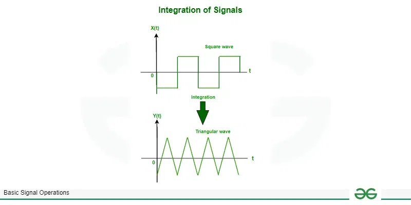
Integration of square wave signal
Basic Signal Operations Performed on Time
Basic operations on independent variable time are also known as Time transformations. In which we manipulate or modify the time axis of a signal by applying mathematical operations to its independent variable denoted as ‘ t ‘ while the amplitude of the signal is constant.
There are three basic time domain operations, which are
- Time-Shifting of Signals
- Time-Scaling of Signals
- Time-Reversal or Reflection of Signals
Time-Shifting of Signals
Time shifting is the shifting of the entire signal along the time axis. By applying this operation, shape of the signal remains the same, only the position of the signal changes. It is nothing but the shifting of the origin of the signal.
supposing we have a signal x(t), we modify the time axis of the signal by adding/subtracting a finite value from its independent variable time denoted as ‘ t ‘.
For a continuous time signal
Time shifting by t0 can be denoted as x( t – t0 ).
x( t – t0 ) represents a right shift of the signal along the time axis or we can say x( t – t0 ) is the delayed version of x(t) by t0 where t0 is the positive and real value.
x( t + t0 ) represents a left shift of the signal along the time axis or we can say x( t + t0 ) is the advanced version of x(t) by t0 where t0 is the positive and real value.
For discrete time signals : same concept as for continuous time signal.
Time shifting by n0 can be denoted as x[n – n0] where n0 is an integer value.
Example: x(t) be a signal shown below. find x( t-2 ) and x( t+1 ).

example on time shifting
x(t) = 1 ; [Tex]-4 \leq t \leq 4[/Tex]
0 ; otherwise
put t = t-2 then we get x(t -2)
x(t-2) = 1 ; [Tex]
-4 \leq (t-2) \leq 4 \space or -2 \leq t \leq 6[/Tex]
0 ; otherwise
put t = t+1 then we get x(t +1)
x(t+1) = 1 ; [Tex]
-4 \leq (t+1) \leq 4 \space or -5 \leq t \leq 3[/Tex]
0 ; otherwise
graphically,

solution of example on time shifting
Time-Scaling Operation of Signals
Time scaling is the compression or expansion of the signal on its time axis. It increases or decreases the duration of the existence of the signal. when we manipulate the time axis of a signal by multiplying a constant by its independent variable denoted as ‘ t ‘ . the compression or expansion of the signal depends on a constant or scaling factor.
If the scaling factor is ‘ 𝜶 ‘ then scaled signal can be represented as x( 𝜶t) where 𝜶 is a positive value.
if 𝜶>1 ; then signal will compress by a factor of 𝜶.
0< 𝜶< ; then the signal will expand by a factor of 𝜶.
Example : x(t) be a signal shown below. find x(2t) and x(t/2).

given signal x(t)
x(t) = 1 ; [Tex]
-2 \leq t \leq 2[/Tex]
0 ; otherwise
put t = 2t then we get x(2t )
x(2t) = 1 ; [Tex]
-2 \leq 2t \leq 2 \space or -1 \leq t \leq 1[/Tex]
0 ; otherwise
put t = t/2 then we get x(t /2)
x(t/2) = 1 ; [Tex]
-2 \leq t/2 \leq 2 \space or -4 \leq t \leq 4[/Tex]
0 ; otherwise
graphically,
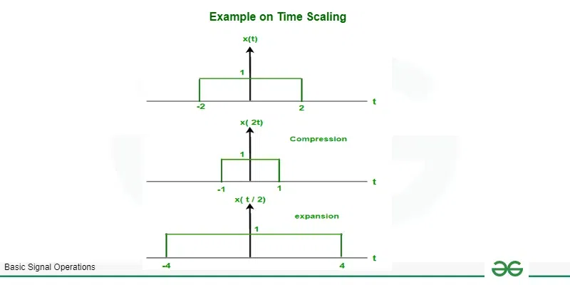
solution of example on time scaling
Time-Reversal of Signals
The time reversal of a signal is the folding of the signal about the vertical axis, or the line t = 0. It is simply taking a mirror image of the signal about the vertical axis. Time reversal and time shifting are both very useful in finding the convolution of signals.
The time reversal of a continuous time signal x(t) can be represented as x(-t)
Note
- Even symmetric signals are not affected by time reversal.
- Whereas time reversal affects odd or asymmetric signals.
Example: x(t) be a signal shown below. find x(-t)?

given signal x(t)
x(t) = 1 ; [Tex]
-2 \leq t \leq 2[/Tex]
0 ; otherwise
put t = -t then we get x(-t )
x(-t) = 1 ; [Tex]
-2 \leq -t \leq 2 \space or -2 \leq t \leq 2[/Tex]
0 ; otherwise
both x(t) and x(-t) are same because x(t) is an Even signal.
graphically,

Example on time reversal
Example : let x(t) be a signal shown below find x(-t)?

given signal x(t)
graphically, we can find out x(-t) by taking mirror image of x(t) about vertical axis.
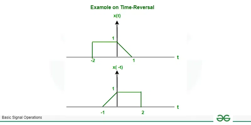
Example on time reversal
Conclusion
In conclusion, Basic signal operations are very important tools for audio, video and image processing, communication systems, control systems etc. We learned basic signal operations performed on dependent amplitude and independent variable time. In which we discussed various types of time transformation like time-shifting of signals, time-scaling of signals, reflection of signals and various amplitude transformations such as amplitude scaling of signals, amplitude reversal, addition of signals, multiplication of signals, differentiation of signals and integration of signals. Throughout our discussion, we used examples to illustrate how these operation are applied in practice.
Basic Signal Operations – FAQs
What do you understand by a time-invariant system?
A system is said to be a time-invariant system if its characteristics do not change with time. i.e., if the input signal is delayed or advanced in time, then the output will also experience the same delay or advancement without changing its characteristics.
What are the classifications of systems?
1) Linear and non-linear systems.
2) Time Variant and Time Invariant systems.
3) Causal and Non causal systems.
4) Static and Dynamic Systems.
5) Stable and Unstable systems.
6) Invertible and Non invertible systems.
What are the steps to convert an analog signal into digital signals?
Step 1 : Sampling – analog signal converted into discrete time and continuous amplitude signal.
Step 2 : Quantization – quantized signal converted into discrete time and discrete amplitude signal or quantized signal.
Step 3 Encoding – quantized signal converted into codewords or digital data and by using line or block coding we can convert digital data into corresponding digital signal.
Share your thoughts in the comments
Please Login to comment...