Admissibility of A* Algorithm

In computer science, the heuristic function h(n) is referred to as acceptable, and it is always less than or equal to the actual cost, which is the true cost from the present point in the path. H(n) is never bigger than h*(n) in this context. This has to do with the idea of reliable heuristics. All reliable heuristics can be used, however not all reliable heuristics can be used.

The cost of reaching the goal state is assessed using an admissible heuristic in an informed search algorithm, however, if we need to discover a solution to the problem, the estimated cost must be lower than or equal to the true cost of reaching the goal state. The algorithm employs the allowable heuristic to determine the best-estimated route from the current node to the objective state.

The evaluation function in A* looks like this:
f(n) = g(n) + h(n)
f(n) = Actual cost + Estimated cost
here, 
            n   = current node.
           f(n) = evaluation function.
           g(n) = the cost from the initial node to the current node.
           h(n) = estimated cost from the current node to the goal state.

Conditions:

h(n) ≤ h*(n) ∴ Underestimation
h(n) ≥ h*(n) ∴ Overestimation

Key Points:

• The heuristic function h(n) is admissible if h(n) is never larger than h*(n) or if h(n) is always less or equal to the true value.
• If A* employs an admissible heuristic and h(goal)=0, then we can argue that A* is admissible.
• If the heuristic function is constantly tuned to be low with respect to the true cost, i.e. h(n) ≤ h*(n), then you are going to get an optimal solution of 100%

Real-Life Examples:

Case 1:  

Let’s suppose, you are going to purchase shoes and shoes have a price of $1000. Before making the purchase, you estimated that the shoes will be worth $1200, When you went to the store, the shopkeeper informed you that the shoe’s actual price was $1, 000, which is less than your estimated value, indicating that you had overestimated their value by $200. so this is the case of Overestimation.

1200 > 1000
i.e. h(n) ≥ h*(n) ∴ Overestimation

Case 2:   

Similar to the last situation, you are planning to buy a pair of shoes. This time, you estimate the shoe value to be $800. However, when you arrive at the store, the shopkeeper informs you that the shoes’ true price is $1000, which is higher than your estimate.indicating that you had understimated their value by $200. In this situation, Underestimation has occurred.

800 < 1000
i.e. h(n) ≤ h*(n) ∴ Underestimation

Example:

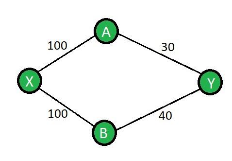
Graph 

where X is the start node and Y is the goal node in between these two nodes there are intermediate nodes A, B and all values which are in the above diagram are actual cost values means h*(n) 

Case 1: Overestimation

Let’s suppose,

H(A)= 60, Estimated values i.e. h(n)]
H(B)= 50  

So, using A* equation, f(n) = G(n) + h(n)   
by putting values

f(A) = 100 + 60 = 160
f(B) = 100 + 50 = 150
by comparing f(A) & f(B), f(A) > f(B) so choose path of B node and apply A* equation again

f(Y) = g(Y) + h(Y) [here h(Y) is 0, Goal state]

= 140 + 0 [g(Y)=100+40=140 this is actual cost i.e. h*(B)]
= 140

The least cost to get from X to Y, as shown in the mentioned graph is 130, however, in Case 1, we took into consideration the expected costs h(n) of A & B, which were 60 & 50, respectively. As a result,  
140 > 130 according to the Overestimation condition h(n) ≥ h*(n), and here, since the value of node f(A) is bigger than f(Y), we are unable to proceed along a different path which is from node A.

Case 2: Underestimation

Let’s suppose,

H(A) = 20 [This are estimated values i.e. h(n)]
H(B) = 10

So, using A* equation, f(n) = G(n) + h(n)  
by putting values

f(A) = 100 + 20 = 120

f(B) = 100 + 10 = 110, by comparing f(A) & f(B), f(A) > f(B), so choose path of B node and apply A* equation again
f(Y) = g(Y) + h(Y) [here h(Y) is 0, because it is goal state]
= 140 + 0 [g(Y) = 100 + 40 = 140 this is actual cost i.e. h*(B)]
= 140

Now, notice that f(Y) is the same in both circumstances but, in 2nd case by comparing the f(A) with f(Y) i.e. 120 < 140 as it means we can go from node A. Therefore A* will go with f(A), which has a value of 120.

f(Y) = g(Y) + h(Y)

= 130 + 0 [g(Y) = 100 + 30 = 130  this is a= 130 + 0 [g(Y) = 100 + 30 = 130  this is actual cost of f(A)]
= 130ctual cost of f(A)]
= 130

So, based on all of these calculations, we can say that this is the optimal value.