What is Forward Propagation in Neural Networks?

Feedforward neural networks stand as foundational architectures in deep learning. Neural networks consist of an input layer, at least one hidden layer, and an output layer. Each node is connected to nodes in the preceding and succeeding layers with corresponding weights and thresholds. In this article, we will explore what is forward propagation and it’s working.

What is Forward Propagation in Neural Networks?

Forward propagation is the process in a neural network where the input data is passed through the network’s layers to generate an output. It involves the following steps:

1. Input Layer: The input data is fed into the input layer of the neural network.
2. Hidden Layers: The input data is processed through one or more hidden layers. Each neuron in a hidden layer receives inputs from the previous layer, applies an activation function to the weighted sum of these inputs, and passes the result to the next layer.
3. Output Layer: The processed data moves through the output layer, where the final output of the network is generated. The output layer typically applies an activation function suitable for the task, such as softmax for classification or linear activation for regression.
4. Prediction: The final output of the network is the prediction or classification result for the input data.

Forward propagation is essential for making predictions in neural networks. It calculates the output of the network for a given input based on the current values of the weights and biases. The output is then compared to the actual target value to calculate the loss, which is used to update the weights and biases during the training process.

Mathematical Explanation of Forward Propagation

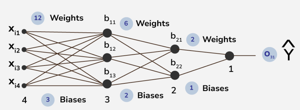
• In the above picture , the first layer of [Tex]X_{i1} , X_{i2} , X_{i3} , X_{i4}[/Tex] are the input layer and last layer of [Tex]b_{31}[/Tex] is the output layer .
• Other layers are hidden layers in this structure of ANN . this is a 4 layered deep ANN where first hidden layer consists of 3 neuron and second layer consists of 2 neuron .
• There are total 26 trainable parameters . here , in hidden layer 1 , the top to bottom biases are [Tex]b_{11} , b_{12} , b_{13}[/Tex] and in hidden layer 2 , the top to bottom biases are [Tex]b_{21}, b_{22}[/Tex] . the output layer contains the neuron having bias b31 . likewise the weights of corresponding connections are assigned like [Tex]W_{111}, W_{112}, W_{113} , W_{121}, W_{122} [/Tex]etc.
• Here, considering we are using sigmoid function as the activation function

The output prediction function is: [Tex]\sigma(w^\Tau x+ b)[/Tex]

Inside Layer 1

Here, from the previous output function , weights and biases are segmented as matrices and the dot product has been done along with matrix manipulation .

The procedure of the matrix operations for layer 1 are as follows:

[Tex]\sigma\left(\begin{bmatrix} W_{111} & W_{112} & W_{113} \\ W_{121} & W_{122} & W_{123} \\ W_{131} & W_{132} & W_{133} \\ W_{141} & W_{142} & W_{143} \end{bmatrix}^T \begin{bmatrix} X_{i1} \\ X_{i2} \\ X_{i3} \\ X_{i4} \end{bmatrix} + \begin{bmatrix} b_{11} \\ b_{12} \\ b_{13} \end{bmatrix}\right) = \sigma\left(\begin{bmatrix} W_{111}X_{i1} + W_{121}X_{i2} + W_{131}X_{i3} + W_{141}X_{i4} \\ W_{112}X_{i1} + W_{122}X_{i2} + W_{132}X_{i3} + W_{142}X_{i4} \\ W_{113}X_{i1} + W_{123}X_{i2} + W_{133}X_{i3} + W_{143}X_{i4} \end{bmatrix} + \begin{bmatrix} b_{11} \\ b_{12} \\ b_{13} \end{bmatrix}\right) = \sigma\left(\begin{bmatrix} W_{111}X_{i1} + W_{121}X_{i2} + W_{131}X_{i3} + W_{141}X_{i4} + b_{11} \\ W_{112}X_{i1} + W_{122}X_{i2} + W_{132}X_{i3} + W_{142}X_{i4} + b_{12} \\ W_{113}X_{i1} + W_{123}X_{i2} + W_{133}X_{i3} + W_{143}X_{i4} + b_{13} \end{bmatrix}\right) = \begin{bmatrix} O_{11} \\ O_{12} \\ O_{13} \end{bmatrix} = a^{[1]} [/Tex]

After the completion of the matrix operations, the one-dimensional matrix has been formed as [Tex] \begin{bmatrix} O_{11} & O_{12} & O_{13} \end{bmatrix} [/Tex]which is continued as $a^{[1]}$ known as the output of the first hidden layer.

Inside Layer 2

[Tex]\sigma\left(\left[\begin{array}{cc} W_{211} & W_{212} \\ W_{221} & W_{222} \\ W_{231} & W_{232} \end{array}\right]^T \cdot \left[\begin{array}{c} O_{11} \\ O_{12} \\ O_{13} \end{array}\right] + \left[\begin{array}{c} b_{21} \\ b_{22} \end{array}\right]\right) \\ = \sigma\left(\left[\begin{array}{cc} W_{211} \cdot O_{11} + W_{221} \cdot O_{12} + W_{231} \cdot O_{13} \\ W_{212} \cdot O_{11} + W_{222} \cdot O_{12} + W_{232} \cdot O_{13} \end{array}\right] + \left[\begin{array}{c} b_{21} \\ b_{22} \end{array}\right]\right) \\ = \sigma\left(\left[\begin{array}{c} W_{211} \cdot O_{11} + W_{221} \cdot O_{12} + W_{231} \cdot O_{13} + b_{21} \\ W_{212} \cdot O_{11} + W_{222} \cdot O_{12} + W_{232} \cdot O_{13} + b_{22} \end{array}\right]\right) \\ = \left[\begin{array}{c} O_{21} \\ O_{22} \end{array}\right] \\ = a^{[2}] [/Tex]

The output of the first hidden layer and the weights of the second hidden layer will be computed under the previously stated prediction function which will be matrix manipulated with those biases to give us the output of the second hidden layer i.e. the matrix [Tex]\left[ O_{21} \quad O_{22} \right] [/Tex]. The output will be stated as [Tex]a^{[2]} [/Tex]here:

Inside Output Layer

[Tex]\sigma\left(\left[\begin{array}{c} W_{311} \\ W_{321} \end{array}\right]^T \cdot \left[\begin{array}{c} O_{21} \\ O_{22} \end{array}\right] + \left[ b_{31} \right]\right) \\ = \sigma\left(\left[W_{311} \cdot O_{21} + W_{321} \cdot O_{22}\right] + \left[ b_{31} \right]\right) \\ = \sigma\left(W_{311} \cdot O_{21} + W_{321} \cdot O_{22} + b_{31}\right) \\ = Y^{i} = \left[ O_{31} \right] \\ = a^{[3]} [/Tex]

like in first and second layer , here also matrix manipulation along with the prediction function takes action and present us a prediction as output for that particular guessed trainable parameters in form of [Tex]\left[ O_{31} \right] [/Tex] which is termed as[Tex]a^{[3]} = Y^{i} [/Tex] here.

Now as for the complete equation , we can conclude as follows :

[Tex]\sigma(a[0]*W[1] + b[1]) = a[1] \sigma(a[1]*W[2] + b[2]) = a[2] \sigma(a[2]*W[3] + b[3]) = a[3][/Tex]

which concludes us to :

[Tex]\sigma(\sigma((\sigma(a[0]*W[1] + b[1])*W[2] + b[2])*W[3] + b[3]) = a[3][/Tex]

Steps for Forward Propagation in Neural Network

The steps can be described at once as:

Step 1: Parameters Initialization

• We will first initialize the weight matrices and the bias vectors. It’s important to note that we shouldn’t initialize all the parameters to zero because doing so will lead the gradients to be equal and on each iteration the output would be the same, and the learning algorithm won’t learn anything.
• Therefore, it’s important to randomly initialize the parameters to a value between 0 and 1. The learning rate will be recommended as 0.01 to make the activation function active.

Step 2: Activation function

There is no definitive guide for which activation function works best on specific problems, based on specific requirements activation function must be choosen.

Step 3: Feeding forward

Given inputs from the previous layer, each unit computes an affine transformation [Tex]𝑧=𝑊𝑇𝑥+𝑏[/Tex] and then applies an activation function [Tex]𝑔(𝑧) [/Tex]such as ReLU element-wise. During this process, we will store all the variables computed and used on each layer to be used in backpropagation.

Implementation of Forward Propagation in Neural Networks

In this section, we are going to implement basic components of neural network and demonstrate how data flows through the network, from input to output, by performing forward propagation. We have discussed the points below:

1. Importing Modules: It imports the necessary libraries, NumPy and Pandas.
2. Creating Dataset: It creates a DataFrame df with columns ‘cgpa’, ‘profile_score’, and ‘lpa’.
3. Initialize Parameters Function (initialize_parameters): This function initializes the weights W and biases b for each layer of the neural network. It returns a dictionary containing the initialized parameters.
4. Forward Propagation Functions (linear_forward, L_layer_forward): These functions perform the forward pass through the neural network. linear_forward computes the linear transformation [Tex]𝑍=𝑊𝑇⋅𝐴_{prev}+𝑏[/Tex], while L_layer_forward iterates through the layers, applying the linear transformation and activation function to compute the output of the network.
5. Example Execution: It demonstrates an example execution of the forward pass for the first row of the dataset df, using the initialized parameters.

Python3

import numpy as np import pandas as pd # Creating a dataset df = pd.DataFrame([[8, 8, 4], [7, 9, 5], [6, 10, 6], [5, 12, 7]], columns=['cgpa', 'profile_score', 'lpa']) # Initializing parameters def initialize_parameters(layer_dims): np.random.seed(3) parameters = {} L = len(layer_dims) for i in range(1, L): parameters['W' + str(i)] = np.ones((layer_dims[i-1], layer_dims[i])) * 0.1 parameters['b' + str(i)] = np.zeros((layer_dims[i], 1)) return parameters # Forward propagation def linear_forward(A_prev, W, b): Z = np.dot(W.T, A_prev) + b return Z def relu(Z): return np.maximum(0, Z) def L_layer_forward(X, parameters): A = X caches = [] L = len(parameters) // 2 for i in range(1, L): A_prev = A W = parameters['W' + str(i)] b = parameters['b' + str(i)] Z = linear_forward(A_prev, W, b) A = relu(Z) cache = (A_prev, W, b, Z) caches.append(cache) # Output layer W_out = parameters['W' + str(L)] b_out = parameters['b' + str(L)] Z_out = linear_forward(A, W_out, b_out) AL = Z_out return AL, caches # Example execution X = df[['cgpa', 'profile_score']].values[0].reshape(2, 1) parameters = initialize_parameters([2, 2, 1]) y_hat, caches = L_layer_forward(X, parameters) print("Final output:") print(y_hat)

Output:

Final output: [[0.32]]

Neural networks learn complex relationships by introducing non-linearity at each layer, combining different proportions of the output curve to minimize loss. Trainable parameters (weights and biases) are adjusted through backpropagation, a process of continuously assigning new values to them to minimize the deviation between the predicted and actual results over multiple epochs. Forward propagation is the foundational step of backpropagation, where inputs are passed through the network to generate predictions.