Convolutional neural networks are very powerful in image classification and recognition tasks. CNN models learn features of the training images with various filters applied at each layer. The features learned at each convolutional layer significantly vary. It is an observed fact that initial layers predominantly capture edges, the orientation of image and colours in the image which are low-level features. With an increase in the number of layers, CNN captures high-level features which help differentiate between various classes of images.
To understand how convolutional neural networks learn spatial and temporal dependencies of an image, different features captured at each layer can be visualized in the following manner.
Considering a dataset with images of cats and dogs, we build a convolutional neural network and add a classifier on top of it, to recognize the image given as either a cat or a dog.
Step 1: Loading the dataset and preprocessing the data
Training images and Validation images are loaded into a data generator using Keras ImageDataGenerator.
The class mode is considered as ‘Binary’ and Batch size is considered as 20. The target size of the image is fixed as (150, 150).
from keras.preprocessing.image import ImageDataGenerator
train_datagen = ImageDataGenerator(rescale = 1./255)
test_datagen = ImageDataGenerator(rescale = 1./255)
train_generator = train_datagen.flow_from_directory(train_img_path, target_size =(150, 150),
batch_size = 20, class_mode = "binary")
validation_generator = test_datagen.flow_from_directory(val_img_path, target_size =(150, 150),
batch_size = 20, class_mode = "binary")
|
Step 2: Architecture of the model
A combination of two-dimensional convolutional layers and max-pooling layers are added, a dense classification layer is also added on top of it. For the final Dense layer, Sigmoid activation function is used as it is a two-class classification problem.
from keras import models
from keras import layers
model = models.Sequential()
model.add(layers.Conv2D(32, (3, 3), activation ='relu', input_shape =(150, 150, 3)))
model.add(layers.MaxPooling2D((2, 2)))
model.add(layers.Conv2D(64, (3, 3), activation ='relu'))
model.add(layers.MaxPooling2D((2, 2)))
model.add(layers.Conv2D(128, (3, 3), activation ='relu'))
model.add(layers.MaxPooling2D((2, 2)))
model.add(layers.Conv2D(128, (3, 3), activation ='relu'))
model.add(layers.MaxPooling2D((2, 2)))
model.add(layers.Flatten())
model.add(layers.Dense(512, activation ='relu'))
model.add(layers.Dense(1, activation ="sigmoid"))
model.summary()
|
Output: Model Summary
Model: "sequential_1"
_________________________________________________________________
Layer (type)                 Output Shape              Param #
=================================================================
conv2d_1 (Conv2D)            (None, 148, 148, 32)      896
_________________________________________________________________
max_pooling2d_1 (MaxPooling2 (None, 74, 74, 32)        0
_________________________________________________________________
conv2d_2 (Conv2D)            (None, 72, 72, 64)        18496
_________________________________________________________________
max_pooling2d_2 (MaxPooling2 (None, 36, 36, 64)        0
_________________________________________________________________
conv2d_3 (Conv2D)            (None, 34, 34, 128)       73856
_________________________________________________________________
max_pooling2d_3 (MaxPooling2 (None, 17, 17, 128)       0
_________________________________________________________________
conv2d_4 (Conv2D)            (None, 15, 15, 128)       147584
_________________________________________________________________
max_pooling2d_4 (MaxPooling2 (None, 7, 7, 128)         0
_________________________________________________________________
flatten_1 (Flatten)          (None, 6272)              0
_________________________________________________________________
dense_1 (Dense)              (None, 512)               3211776
_________________________________________________________________
dense_2 (Dense)              (None, 1)                 513
=================================================================
Total params: 3, 453, 121
Trainable params: 3, 453, 121
Non-trainable params: 0
Step 3: Compiling and training the model on cats and dogs dataset
Loss function: Binary cross Entropy
Optimizer: RMSprop
Metrics: Accuracy
from keras import optimizers
model.compile(loss ="binary_crossentropy", optimizer = optimizers.RMSprop(lr = 1e-4),
metrics =['accuracy'])
history = model.fit_generator(train_generator, steps_per_epoch = 100, epochs = 30,
validation_data = validation_generator, validation_steps = 50)
|
Step 4: Visualizing intermediate activations (Output of each layer)
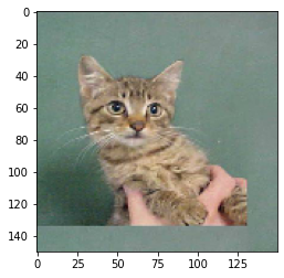
Consider an image which is not used for training, i.e., from test data, store the path of image in a variable ‘image_path’.
from keras.preprocessing import image
import numpy as np
img = image.load_img(image_path, target_size = (150, 150))
img_tensor = image.img_to_array(img)
img_tensor = np.expand_dims(img_tensor, axis = 0)
img_tensor = img_tensor / 255.
print(img_tensor.shape)
import matplotlib.pyplot as plt
plt.imshow(img_tensor[0])
plt.show()
|
Output:
Tensor shape:
(1, 150, 150, 3)

Input image:
Code: Using Keras Model class to get outputs of each layer
layer_outputs = [layer.output for layer in model.layers[:8]]
activation_model = models.Model(inputs = model.input, outputs = layer_outputs)
activations = activation_model.predict(img_tensor)
first_layer_activation = activations[0]
print(first_layer_activation.shape)
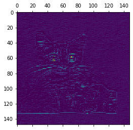
plt.matshow(first_layer_activation[0, :, :, 6], cmap ='viridis')
plt.matshow(first_layer_activation[0, :, :, 15], cmap ='viridis')
|
Output:
First layer activation shape:
(1, 148, 148, 32)

Sixth channel of first layer activation:


Fifteenth channel of first layer activation:
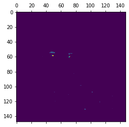
As already discussed, initial layers identify low-level features. The 6th channel identifies edges in the image, whereas, the fifteenth channel identifies the colour of the eyes.
Code: The names of the eight layers in our model
layer_names = []
for layer in model.layers[:8]:
layer_names.append(layer.name)
print(layer_names)
|
Output:
Layer names:

['conv2d_1',
 'max_pooling2d_1',
 'conv2d_2',
 'max_pooling2d_2',
 'conv2d_3',
 'max_pooling2d_3',
 'conv2d_4',
 'max_pooling2d_4']
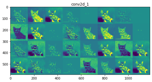
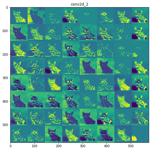
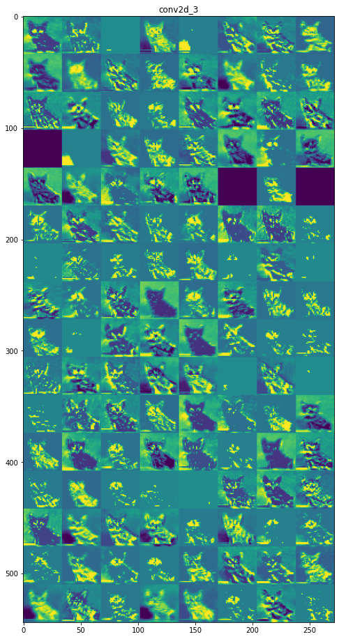
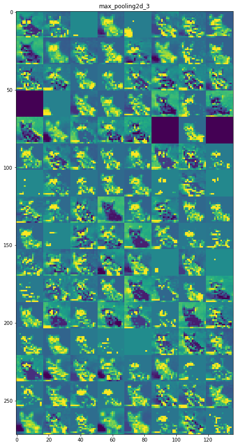
Feature maps of each layer:
Layer 1: conv2d_1
Layer 2: max_pooling2d_1

Layer 3: conv2d_2
Layer 4: max_pooling2d_2

Layer 5: conv2d_3
Layer 6: max_pooling2d_3
Layer 7: conv2d_4

Layer 8: max_pooling2d_4

Inference:
Initial layers are more interpretable and retain the majority of the features in the input image. As the level of the layer increases, features become less interpretable, they become more abstract and they identify features specific to the class leaving behind the general features of the image.
References:
- https://keras.io/api/models/model/
- https://www.kaggle.com/c/dogs-vs-cats
- https://www.geeksforgeeks.org/introduction-convolution-neural-network/
Share your thoughts in the comments
Please Login to comment...