Top Excel Data Cleaning Techniques to Know in 2024

In the world of business and data analysis, being a pro at Excel Data Cleaning is a game-changer. Everyone wants top-notch accuracy and quality in data, right? Well, that’s where Excel comes in handy! Cleaning up your data involves kicking out those pesky blank spaces, fixing mistakes, and updating outdated info.

You can do all of this super easily using Excel Power Query. This tutorial is your go-to guide for mastering the basics of cleaning up your data in Excel. We’re keeping it simple, so you’ll be data-cleaning within no time! Ready to make your data sparkle? Let’s dive in!

What is Data Cleaning in Excel

Most of the time the data you want to analyze on is not in a usable format i.e., it contains blank cells, duplicate values, merged columns, etc. Before using this data for analysis we need to clean it so that it does not provide any irrelevant results. It ensures accuracy and reliability in your analyses. 

How to Clean Data in Excel?

Excel provides some techniques to do data cleaning easily. The most widely used techniques are :

Remove Duplicates

This is a common issue that can occur when data is copied and pasted from multiple sources. Excel has a built-in function to remove duplicates, which can save you a lot of time and effort.

Standardize Formats

Inconsistent formatting can make it difficult to analyze your data. You can use Excel’s formatting tools to standardize the format of your data, such as currency, dates, and times.

Clean Text Data

Text data can often contain errors, such as typos, extra spaces, and inconsistent capitalization. You can use Excel’s cleaning tools to fix these errors. Some common functions used for cleaning text data include TRIM, CLEAN, and PROPER.

Fill Missing Values

Missing values can also occur in your data. You can use Excel’s data analysis tools to fill in missing values, such as the average or median of the surrounding data.

Data Validation

Data validation can help to prevent errors from being entered into your data in the first place. You can use data validation to specify the type of data that can be entered into a cell, as well as the range of valid values.

Conditional Formatting

Conditional formatting can be used to highlight errors in your data. For example, you can use conditional formatting to highlight cells that contain blank values or invalid characters.

Power Query

Power Query is a powerful tool that can be used to clean and transform your data. Power Query can be used to import data from a variety of sources, clean and transform the data, and then load the data into an Excel table.

Note: It’s crucial to always back up your data before performing any significant cleaning operations as they may result in irreversible changes.

How to Remove Duplicates in Excel

One simple method for cleaning data in Excel involves removing duplicate entries. It’s quite possible for data to unintentionally contain duplicates without the user realizing it. In such cases, you can easily eliminate these duplicate values.

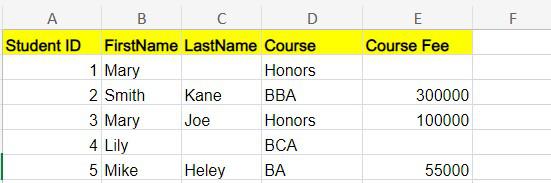
For instance, let’s take a basic student dataset with duplicate values. You can utilize Excel’s built-in function to remove these duplicates, as demonstrated below.

Example: In this example, the entries for Student ID 1 and Student ID 3 are duplicates because they have the same values in the FirstName, LastName, Course, and Course Fee columns. You can remove the duplicated data with the following steps:

Duplicate Data is present in the table

Step 1: Go to the Data tab and click on Remove Duplicates

Navigate to the Data Tab and select “Remove Duplicates” to easily eliminate identical entries

GO to the Data Tab and Click on Remove Duplicates

Step 2: Select All Columns and click OK

In this case, we want to remove duplicates based on all columns that’s why choose “Select all Columns” and click “OK”.

“Select all Columns” > OK

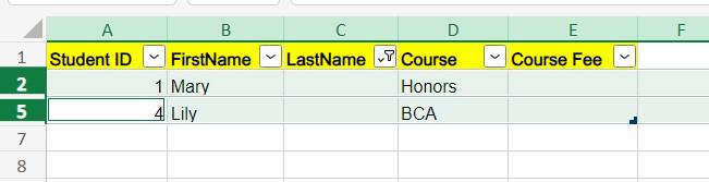
You will get the following pop-up window for the deletion of 1 duplicate record:

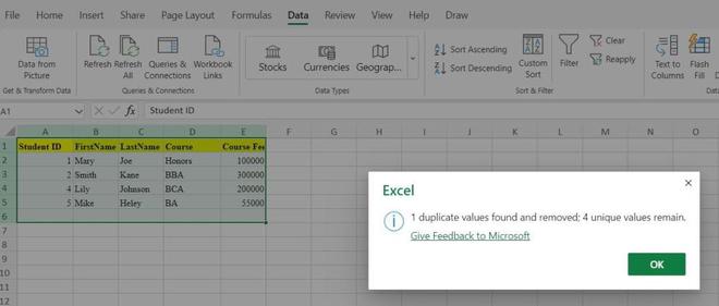
Our data contained only 1 duplicate value.

Step 3: Preview Results

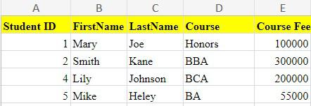
Final data after removing duplicates

How to Parse Data in Excel

This feature in Excel is useful when you have data in a single column that you want to split into multiple columns. This is particularly handy when dealing with data imported from external sources, such as CSV files, or when data is not organized in a way that suits your analysis.

Example: Consider a dataset where you have to split FullName into FirstName and LastName:

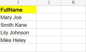
Splitting FullName to FirstName and LastName

Step 1: Select all data then go to the Data tab and click on “Text to Columns”.

We need to select the data on which we have to apply Text to Columns then navigate to the Data tab and select Text to Columns under Data Tools.

“Data” > “Text to Columns”

Step 2: Choose Space as delimiter and click OK

Here, we need to split out data based on the space between them. That’s why chose space as a delimiter.

“Space” > “Apply”

Step 3: Preview Result

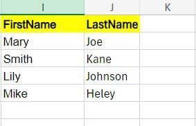
Final data after splitting the column

TRIM Function – Remove Extra Spaces in Excel

The TRIM function in Excel is used to remove extra spaces from a text string, leaving only a single space between words and no leading or trailing spaces.

Example: From the following data we need to remove extra spaces and we can do it using the TRIM() function in Excel.

Step 1: Write the TRIM formula

The trim function will remove the extra spaces from L2 and the result will be visible in cell M2.

=TRIM(L2)

=TRIM(L2)

Step 2: Copy Formulas with the Fill Handle

Then, drag the fill handle (a small square at the bottom-right corner of the cell) down to copy the formula for the entire range. 

Step 3: Preview Result 

The final Data should look like the below

Final data after trimming

How to Use Find & Replace to Clean Data in Excel

The “Find and Replace” feature in Excel is handy for quickly locating specific data and replacing it with new values. This can be useful for correcting errors, updating information, or making changes to a large dataset.

Example: From the following data we need to remove and replace the errors.

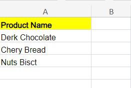
Error in Data

Step 1: Enter Ctrl+H to launch the “Find and Replace” window

A window will open asking you to replace the word. You can enter the word to replace and the word with whom you need to replace.

Step 2: Click on Replace all after entering the data.

Enter Derk in “Find” and Dark in “Replace with”. Click “Replace” to replace the word.

“Replace All”

Step 3: Repeat Step 1 and Step 2

Replacing Chery with Cherry

Replacing Bisct with Biscuit

Step 3: Preview Result

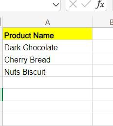
Final data after replacing the errors

How to Select & Treat all Blank Cells

Removing blank rows in Excel is a straightforward process and can be done using filters or a special function.

Example: Consider the following data which contains four blank spaces. It can be removed by following steps:

Blank cells in Lastname and Course Fee

Step 1: Go Home tab then navigate to Sort & Filter and choose Filter.

You need to select the whole data and then click on the Home tab. After that choose Filter under Sort & Filter. An arrow sign will appear on each column heading.

Select all Data > “Sort & Filter” > Filter

Step 2: Deselect all the columns and only select the (Blanks) column. Click Apply.

We need to check the blank cells in the data. For this purpose select the blanks checkbox.

Step 3: Select and delete the rows in blank rows.

Records with blank cells will appear. Select the data and delete them to get rid of the blank records.

Deleting Blank rows

Step 4: Choose Select All and click Apply

To see the records left after deleting the blank cells click on Select All and Apply the changes.

Select All

Step 5: Preview Result

Final output

How to Use Data Validation in Excel

Data validation in Excel is a powerful tool that allows you to set rules or criteria for the data entered into a cell or range of cells. This can be particularly useful for ensuring data accuracy and consistency.

Example: Consider the following data in which the Age column contains -ve and invalid decimal age value. We can solve this using the following steps:

-ve and decimal value in the Age Column

Step 1: Go to the Data tab and select “Data Validation”.

Select the records in the Age column and navigate to Data Validation under the Data tab to add validation to the Age columns.

“Data” > “Data Validation”

Step 2: Enter the Validations

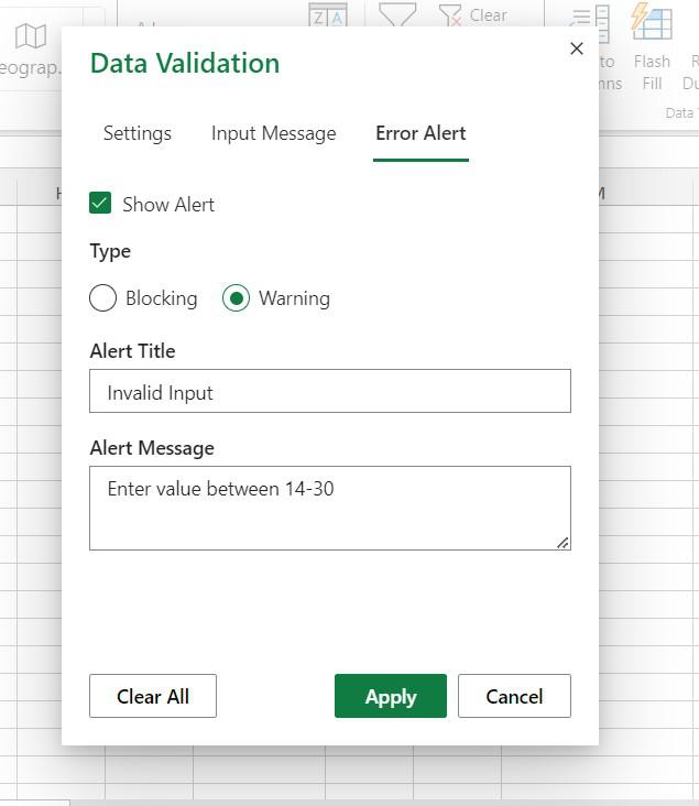
Choose “Whole Number” and set the range of Age “Between”, and “14-30”. This will allow users to enter ages of 14 to 30 only. If the user tries to enter age beyond this an error message will appear.

Step 3: Give Input Message

This message will appear when the user hovers on any cell to enter their age. This will guide them on what value is expected in the cell.

Step 4: Give an Error Alert and Click on “Apply”

This Error Alert will appear after the user enters the wrong input in the cell.

Error Alert

How to Convert Numbers Stored as Text into Numbers in Excel

It refers to the process of changing numerical data that is stored as text in a digital format into actual numeric values. Sometimes the numeric data is stored as text due to formatting issues or data import/export processes. This can lead to issues when performing calculations or analyses that require numeric data.

Example: Assume the following numbers are in cells A1 to A6. By default, the data of these numbers are as Text.

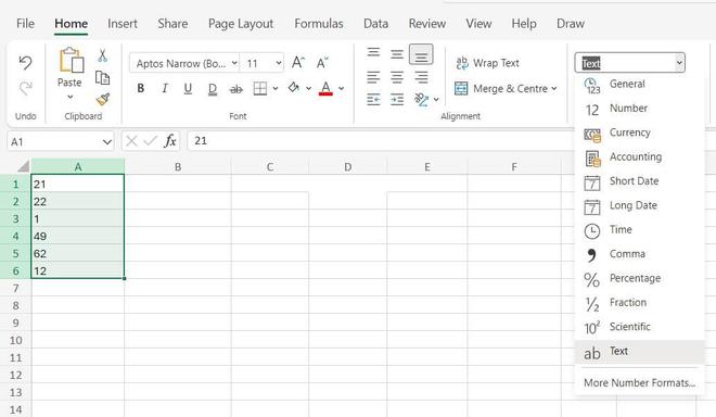
You can check the data type of the cells.

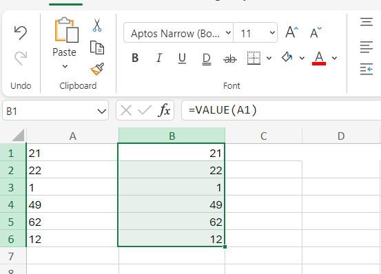
Step 1: Enter the following function in cell B2

=VALUE(A1)

This will change the numerical value in cell A1 wrongly entered as text to Number.

Step 2: Drag the formula to copy it to other cells

Then, drag the fill handle (a small square at the bottom-right corner of the cell) down to copy the formula for the entire range.

Step 3: Preview Result

The final Data should look like below:

How to Highlight Errors in Excel

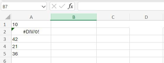
In Excel, you can easily highlight errors in your spreadsheet to quickly identify and correct them. Errors can include things like #DIV/0!, #VALUE!, #REF!, #NAME?, #NUM!, #N/A, or #NULL!. These errors can cause issues when performing calculations or analyses that require numeric data. It is better to deal with these errors before proceeding with further analysis.

Example: Assume you have a column of numbers with some intentional errors. Here’s a sample dataset in column A.

Step 1: Go to the Home tab, click on Conditional Formatting, and then select New Rule.

To highlight the cells with error select the data go to the Home tab and choose New Rule under Conditional Formatting.

Conditional Formatting > New Rules

Step 2: Select the Formatting and click on Done

A window will appear where you can apply the formatting. Choose “Highlight Cells With” and “Errors” under Rule Type. Add the formatting “Light red fill with dark red text”. Click “Apply”

Step 3: Preview Result

Data after highlighting the errors

How to Change Text to Lower/Upper/Proper Case

In Excel, you can easily change the case (lowercase, uppercase, or proper case) of text using built-in functions or formulas. This improves the readability of your data.

Example: Suppose we need to convert the following data to Uppercase/Lowercase/Propercase.

Lower/Upper/Proper Case

1. UPPER Function

Use the UPPER function to convert text to uppercase. Follow the below example:

Example: UPPER

2. LOWER Function

Use the LOWER function to convert it to lowercase. Follow the below example:

Example: LOWER

3. PROPER Function

If you want to convert text to proper case (capitalizing the first letter of each word), use the PROPER function.

Example: Proper

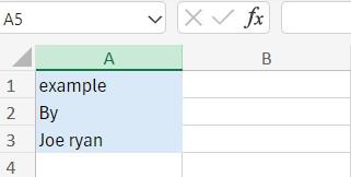
How to Use the Spell Check Feature in Excel

Spell checking in Excel is a useful feature for data cleaning, especially when dealing with text data. It helps identify and correct spelling errors in your spreadsheet.

Example: Consider the below example where the A1 cell has data with the wrong spelling. We can correct it by the following steps:

Spell Check

Step 1: Go to the Review tab and select Spelling

Select the data (A1) which you want to check for spelling. Go to the “Review” tab then select the “Spelling” option. This will provide you with the correct spelling of that word.

Review > Spelling

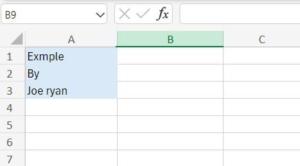
Step 2: Click on the appropriate spelling

The below dialog box will appear after you choose Spelling under the Review tab. Choose the appropriate spelling to replace it with the correct spelling.

Step 3: Preview Result

Final data after using the spell check feature in Excel

Conclusion

In conclusion, data cleaning is an indispensable and transformative process in the realm of data management. It serves as the bedrock for accurate, reliable, and meaningful analyses, ensuring that datasets are free from errors, inconsistencies, and inaccuracies. By addressing issues of completeness, consistency, and accuracy, data cleaning enhances the overall quality of information, facilitating informed decision-making across various domains.

FAQs – Top 5 Excel Data Cleaning Techniques to Know in 2024

What are the best methods for data cleaning in Excel?

Error Checking, Conditional Formatting, Data Validation, Spell Check, Handling Text Case(upper/lower/proper), Handling Text Case and Removing Duplicates are some of the best methods for cleaning the data.

How do I clean data when dealing with extra spaces in Excel?

The TRIM function can be used to remove extra spaces in text data.

How do I split data in a single column into multiple columns in Excel?

Use the “Text to Columns” feature in the “Data” tab to split the columns based on the suitable delimiters.

What is the “Find and Replace” feature in Excel used for?

The “Find and Replace” feature is used to locate specific data in a worksheet and replace it with new values.

Can I use data validation to prevent entering non-numeric values in a column?

Yes, you can. By applying data validation to a column and choosing the appropriate criteria, you can prevent users from entering non-numeric values.