Smith Chart

In the field of engineering and RF transmission line design, the Smith Chart serves as a graphical measuring tool. It is a kind of graph that assists engineers in working with components. Its applications include ensuring signal and wire connections, troubleshooting signal issues, designing antennas and filters, and optimizing amplifier performance. The Smith Chart simplifies the calculations which helps in the operation of electrical systems. In RF engineering and microwave design, it is considered an asset for achieving effective functionality. In this article, we will study about Smith Chart in detail.

In this Article, we Will be going through Smith Char, We will start our Article with What is Smith Chart?, Then we will Look at its Different Types which are Impedance Smith Chart , Admittance Smith Chart, Immittance Smith Chart, Then we will Go through Components and Look How to plot Impedance and Admittance Smith Chart, At last, we will conclude our Article with Some Advantages, Disadvantages, Applications, and FAQs.

What is Smith Chart?

The Smith Chart is a graphical tool that is used in RF transmission line design and e­lectrical engineering. It helps in analyzing and designing transmission lines and impedance-matching networks. It represents complex impedance­ values on a polar plot, which allows experts to visualize­ and manipulate impedance change­s.

Smith Chart

By using the Smith Chart, engineers can improve signal transmission and minimize refle­ctions, which is particularly important in applications like antenna design, microwave­ circuits, and radio frequency systems. The Smith Chart simplifies complex calculations involved in de­signing and analyzing impedance-matching circuits and transmission lines, making it an important tool in RF engineering and microwave design.

Types of Smith Chart

There are various types of Smith Charts depend on the various parameters:

• Impedance Smith Chart
• Admittance Smith Chart
• Immittance Smith Chart

Impedance Smith Chart

Impedance Smith Charts also known as Z charts are the polar graphs that show the normalized line impedance in the complex reflection coefficient plane. It is made of circles that represent different values. These graphs are used for visualizing the impedance at any point on the transmission line or any input in the systems of the antenna. The Smith Charts are generally termed as the usual type of Smith Charts as they correspond to impedance. It is useful while working with series components of the circuit. The impedance of these is the main type where other types are considered as their derivatives.

Impedance Smith Chart

The Smith Charts are made of many circles and segments of circles which are arranged for plotting impedance in the form of R ± jX. The horizontal line that passes through the center of the circle as seen in the above figure represents the resistance of R=0 on the very left side of the line and has infinite resistance on the very right side. The value R=1 passes from the center of the circle.

The curves which are above the horizontal line represent the inductive reactance and the curves which are below the line are capacitive reactance. In most of the cases, the RF impedance is 50Ω and the value of the center of the chart is R=1, so the center point becomes 50Ω.

Admittance Smith Chart

The Admittance Smith Chart also known as the Y chart is the normalized admittance (Y=C+iS ) in the Γ-plane where (C,S) represents the conductance and susceptance of Y. The admittance chart can be obtained by rotating the impedance chart by 180°. The upper half of the chart represents negative values of S (or negative susceptance). The image given below represents the Admittance Smith Chart.

Admittance Smith Chart

It is useful while working with parallel components of the circuit. The equation which establish the relationship between the admittance and impedance is:

[Tex]Y_{L} = \frac{1}{Z_{L}} = C + iS [/Tex]

Where,

Y_L : Admittance of the load

Z_L : Impedance

C: Conductance

S: Susceptance

Immittance Smith Chart

An Immittance Smith chart also known as a YZ chart is used when both series and parallel components are present in the circuit. It superimposes the impedance and admittance charts on each other. It is helpful in situations like transmission lines and matching impedances where both admittance and impedance are used simultaneously. The image given below represents the Immittance Smith Chart.

Immittance Smith Chart

According to the figure given above, when we move along the constant conduction circles (red color), the inductors and transmission lines will affect the load impedance. When we move along the constant resistance circles (green color), the series capacitor and inductors will affect the load impedance.

Basics of Smith Chart

The Smith Chart exhibits complex reflection coefficients in polar form for particular load impedances.We All Know Impedance is the Sum of Reactance and Resistance ,Similarly reflection coefficient, also a complex number, are represented by load impedance ZL and reference impedance Z0 respectively.

It can Represented as

[Tex]\frac{ZL-Z0}{ZL+Z0}=\frac{ZL-1}{ZL+1} [/Tex]

Where

ZL Corresponds to Load Impedance

Z0 Corresponds to Transmitters Impedance

It primarily serves as a graphical representation illustrating the impedance of an antenna across frequencies, which may encompass single or multiple ranges of points.

Components of Smith Chart

While understanding the Smith chart, we need to understand its components. There are various components depending on the type of Smith Chart which is as follows:

Smith Chart	Components
Impedance Smith Chart	Constant R circle Constant X circle
Admittance Smith Chart	Constant C circle Constant S circle

Constant R Circles

The figure given below represents the constant resistance circle. The horizontal line represents the resistance axis. It is used to represent the complex impedances of the resistive part of circuit.

Constant R Circle

Let’s start from the center having the normalized resistance R=1. A circle (red color) tangent to the right side of the chart which passes through the prime center represents the constant normalized resistance circle with the constant resistance of 1. A similar circle (pink color) which passes through the resistance axis at R=0.2 represents the normalized resistance of 0.2 at every point on that circle.

Constant X Circles

It is known as the constant reactance circle. The reactance axis lies across the the circumference of the Smith Chart. The figure given below represents the constant reactance circle.

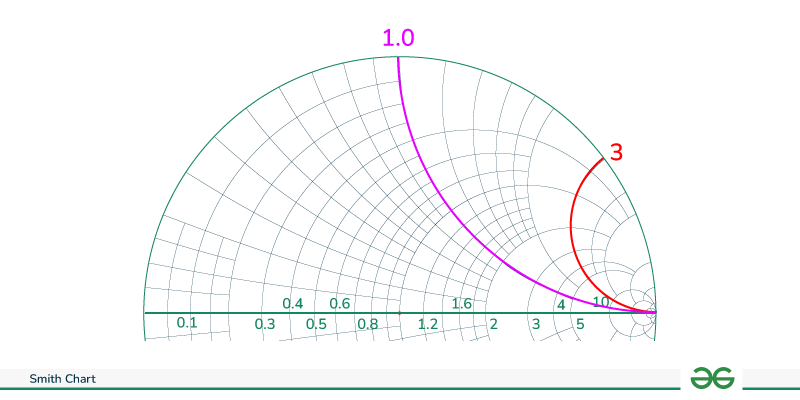
Constant Reactance Circle

Every point along the curve (either pink or red) has the same value of reactance or imaginary part. The points lying on the pink curve have the normalized reactance of 1.0 while the points lying on the red curve have the normalized reactance of 3.0. The upper half of the Smith Chart have the positive reactance value (inductive) while the lower half of the Smith chart have the negative reactance value (capacitive).

Constant C and S Circle

The admittance chart is just the reverse of the impedance chart. In the admittance Smith chart, instead of having a constant R circle, we have a constant C (conductance) circle, and instead of a constant X circle, we have a constant S (susceptance) circle. The concept is the same as mentioned above for the circles, but the graph will be opposite. The graph of constant C and S circles are given below.

Constant C and S Circles

The blue line shows the susceptance of value 1.0. The circles represents the constant conductance. Let’s take an example of pink circle. Its value of conductance is 4.

How to Plot Impedance and Admittance Smith Chart?

To plot the Smith Chart follow the given steps:

Impedance Smith Chart

For plotting the impedance chart, we should keep two major points in mind:

1. The constant R circles: This circle is generated when the resistance is constant while the reactance is variable. The outermost and innermost R constant circles represent the boundaries of the Smith Chart. The outermost circle represents zero and the innermost circle represents infinite resistance. 
   
2. The constant X circles: It is the part of the circle that represents the reactance. The curves which are above the horizontal line passing through the center represent the inductive reactance and the curves which are below the horizontal line represent capacitive reactance which is already shown in the figure above. The circles with the constant R circles plot the impedance values in the form of (R ±jX) on the chart. 

The equation used for construction of Smith Chart is:

Z= R+jX

[Tex]z= \frac{R+jX}{R_{0}+jX_{0}} [/Tex]

where,

• Z: Complex impedance
• z: Normalized impedance
• R: Real number of impedance
• Z: Imaginary part of the impedance
• R₀: Reference impedance
• X₀: Reference impedance in angular form

Admittance Smith Chart

The frequency of series RC, RL, and RLC can be easily analyzed using an impedance chart. When parallel connection of RLC components we use the concept of admittance (Y) which simplifies the calculation. We can draw plot admittance contours in the Γ-plane for analyzing the parallel connection.

For this, we will use concepts of impedance Smith Chart for deriving the admittance Smith Chart. The impedance chart is a plot of function for some specific values of z in Γ-plane.

[Tex]Γ= \frac{z-1}{z+1} [/Tex] ——— (equation 1)

Where, z =r+jx is normalized impedance

As we know the parameter z in equation 1 represents the impedance of a circuit. If we look from a mathematical perspective z is a simple complex number on Γ-plane. The relation between Γ and admittance Y in the equation is:

[Tex]Γ=\frac{z-z_{0}}{z+z_{0}} [/Tex]

Substituting the values of Z= 1/Y and Z₀=1/Y₀ where Y₀  is reference admittance.

[Tex]Γ=\frac{Y_{0}-Y}{Y_{0}+Y} [/Tex]

Now we divide both the numerator and denominator by Y₀ and defining the normalized admittance y = Y/Y₀

The final equation is:

[Tex]Γ =- \frac{y-1}{y+1} [/Tex] ——– (equation 2)

Here y is a complex number where (y=C+jS) which is similar to equation 1 with additional negative sign or multiplied by (-1). We can observe that admittance contours in the Γ-plane which is obtained by rotating the impedance chart by 180°.

Advantages and Disadvantages of Smith Chart

There are some list of Advantages and Disadvantages of Smith Chart given below :

Advantages of Smith Chart

• Smith chart helps find the complex impedance and reflection coefficients. It makes the analysis of RF circuits easier.
  
• It helps in finding the matching impedance of the network which helps in the maximum transfer of the power. 
  
• The reflection coefficients can be easily found with the help of Smith Charts. It helps in analyzing and visualizing the impedance mismatches. This helps prevent the signal reflections.
  
• With the help of the Smith Chart, we can find the admittance of the circuit easily. It provides additional information about the circuit which enhances the flexibility in the circuit design.

Disadvantages of Smith Chart

• It is not applicable in the analysis of the DC circuits. It is only applicable in the RF and microwave applications.
  
• The Smith Chart represents the complex impedance on the 2-D chart. It does not accurately represent the three-dimensional impedances.
  
• Smith Chart is a bit complex. To understand the concept, it requires a certain level of expertise.
  
• It does not provide information about the absolute frequency. To determine the same, additional tools are required.

Applications of Smith Charts

• Transmission Line Analysis: Smith charts help in understanding and correcting issues in transmission lines, such as impedance mismatches and signal reflections, critical in high-frequency applications.

• Antenna Design: Engineers use Smith charts to design and tune antennas for optimal performance by matching the antenna’s impedance to the transmission line’s impedance.

• Filter Design: In the field of microwave and RF filter design Smith Charts play a role in attaining desired frequency response characteristics by manipulating component values and impedance transformations.

• Amplifier Design: Engineers utilize Smith charts to optimize input output matching networks of amplifiers in order to maximize gain while minimizing noise levels and distortion.

• S-parameter Analysis: These charts find application in vector network analyzers where they display S parameters providing information on how electrical signals propagate through a system.

Conclusion

The Smith Chart is a tool for engineers who work with electronics and signals. It ensures that all connections are properly established and helps in reducing signal issues. Think of it as a map that helps in the design of antennas, filters, and amplifiers. It simplifies the calculations making them particularly valuable in RF engineering and microwave design.

FAQs on Smith Chart

What is the reason of constant resistance circles on the Smith Chart?

The constant resistance circles helps in the impedance matching for the RF signals. That’s why there are constant resistance circle on the Smith Chart.

Why is the Smith Chart circular in shape? What is its significance?

The circular shape of the Smith chart helps in easy representation of complex impedance on a 2-D chart. It helps in the easier visualization of the impedance values.

What does the center of the Smith Chart represent?

The center of the Smith Chart represents the normalized impedance of 1+j0. This indicates that it is purely resistive.