Simulating electrostatic fields in 2-dimensions using Python3

Last Updated : 24 Oct, 2023

This article shows how to simulate (or trace) electrostatic fields for stationery point charges in 2 dimensions using Python3 programming language and its libraries Matplotlib (for visualization) and NumPy (for handling data in arrays). To work out this article, one needs basic knowledge of Python, Matplotlib and NumPy. Basic knowledge of electrostatics would be helpful but is not absolutely must since the concepts necessary for the program are discussed.

Basics of Electrostatics

Electrostatics is the study of stationary electric charges. We generally visualize point charges in space and then study their interactions with the surroundings and with each other. A point charge is an idealization in which all the charge at a location is concentrated at a point on the location. The magnitude of a charge can be positive or negative.

Coulomb’s Law

The law states that the force (F) between two point charges of magnitudes q₁ and q₂ is given by the formula –

$F = k\frac{q_1\times q_2}{d^2}$ where d is the distance between the charges and k is a constant equal to $9 \times 10^9$ N m²/C².

A positive value indicates a repulsive force while a negative value indicates attractive force.

Electric Field

The electric field (or electrostatic field) of a charge q at a point say p is defined as the force exerted by q on a unit positive charge placed at p. It is mathematically described as –

$E(p) = k\frac{q}{d^2}$ where d is the distance between p and q, q represents the magnitude of the charge, E(p) is the electric field at p due to q.

The electric field of a positive charge is radially outwards and that of a negative charge is radially inwards (in an isolated space). This is shown in the following figures –

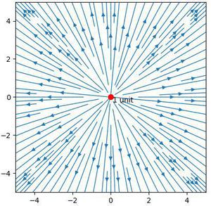
Figure 1: Electric field of a unit positive charge (in isolation)

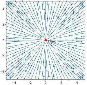
Figure 2: Electric field of a unit negative charge (in isolation)

An electric field line is a curve such that the tangent to it at every point is in the direction of electric field at that point.

Remark: The direction of arrows shows the direction of electric field hence the direction of force experienced by the unit positive charge.

Superposition Principle (for Electric Field)

The superposition principle for electric field states that the electric field at a point p due to a number of charges q1, q2, … qn is equal to the vector sum of electric fields at p due to each of the charges independently. Mathematically –

$E(p) = E_{q1}(p) + E_{q2}(p) + \dots + E_{qn}(p)$

This is an important result that we will be using in the simulation.

Components of an Electric Field

In a 2-dimensional Cartesian system, we can represent a vector as a sum of two vectors – one along (parallel to) x-axis and one along (parallel to) y-axis. These two are called the x and y components of the vector. Now, an electric field is also a vector (since it has both magnitude and direction) hence we can decompose it into its x and y components as well.

This decomposition is important for us because the plotting function we are going to use (matplotlib.pyplot.streamplot) takes two arrays – one containing the x component of the electric field (Ex) and one containing the y component of the electric field (Ey).

Here is the explanation for obtaining Ex and Ey from E (we use some trigonometry here) –

$E_x = E\times \cos(\theta)\newline E_y = E\times \sin(\theta)$ where $\theta$ is the angle between positive direction of x axis and electric field E. This is shown in figures 3.

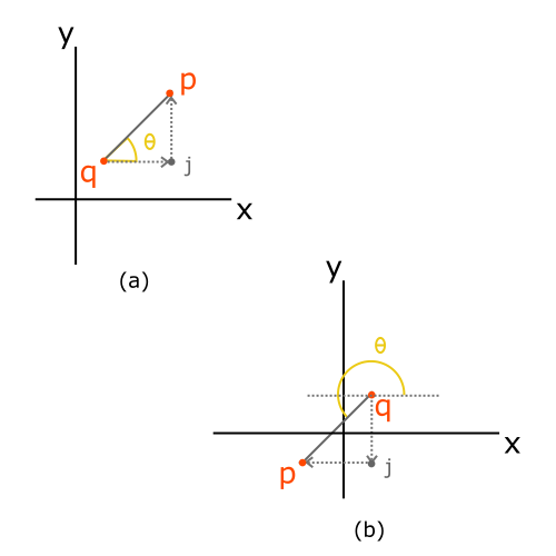
Figure 3: Different configurations between p (point at which electric field is being calculated) and q (point of charge).

The electric field is always parallel to direction qp (as stated earlier) in direction to qp if q is positive and opposite (i.e., pq) if q is negative. This is shown in figure 4.

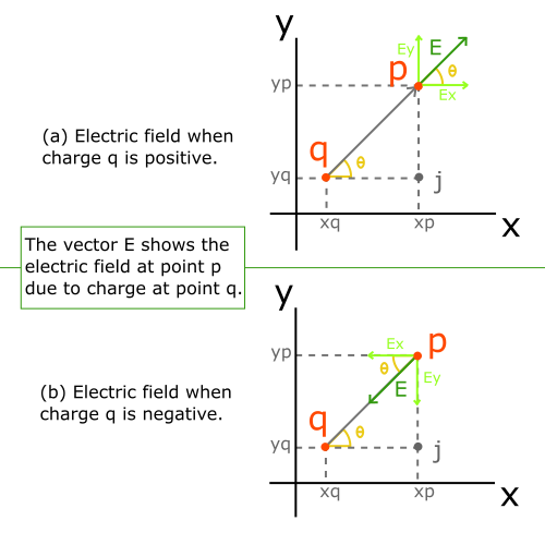
Figure 4: Direction of electric field and its components at point p due to charge at point q.

Calculating sin and cos Values

This section shows how to calculate $\sin(\theta)$ and $\cos(\theta)$ for Ey and Ex. Keeping figure 4 as the reference –

$\sin(\theta) = \frac{height}{hypotenuse} = \frac{jp}{|qp|} = \frac{y_p - y_q}{\sqrt{(x_p - x_q)^2 + (y_p - y_q)^2}}$

$\cos(\theta) = \frac{base}{hypotenuse} = \frac{qj}{|qp|} = \frac{x_p - x_q}{\sqrt{(x_p - x_q)^2 + (y_p - y_q)^2}}$

Note that the above formula works for all configurations of p and q (whether it is like Fig.3 (a) or Fig.3 (b) or whatever). This is just simple vector math. Look at figure 5 below –

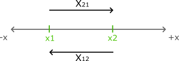
Figure 5: Shows how x21 is different from x12

$x_{21}$ represents length to x2 starting from x1. Similarly, $x_{12}$ represents length to x1 starting from x2. Note that $x_{12} = -x_{21} \space \& \space |x_{12}| = |x_{21}|$ . These can be obtained as follows –

$x_{12} = x_1 - x_2\newline x_{21} = x_2 - x_1$

Similarly, direction can be obtained on y-axis too. Since location of x1 and x2 (equivalently y1 and y2 on y-axis) doesn’t matter in above formula, therefore the formula for sin and cos are universal on 2d plane (i.e., work for any locations of p and q).

Algorithm for the Python Code

With the above theory, we proceed to the algorithm for the simulation (the comments inside ‘[ ]’ explain the algorithm where necessary)-

1. Divide the sample area into M rows and N columns

(thus obtaining MxN sample points)

2. Let x be a MxN array such that x[j][i] = x coordinate of sample-point[j][i].

3. Let y be a MxN array such that y[j][i] = y coordinate of sample-point[j][i].

4. Let Q be the list of charges with each element containing x,y coordinates and magnitude of the corresponding charge.

5. Let Ex and Ey be two MxN arrays with all the values initiated to 0.

6.

[Now we start filling Ex and Ey such that

Ex[j][i] = x component of the electric field at sample-point[j][i] and

Ey[j][i] = y component of the electric field at sample-point[j][i]

]

for j from 1 to N:

for i from 1 to M:

for each C in Q:

[each loops adds the electric field contribution from a charge in Q on sample point [j][i] until all charges are done, superposition principle]

deltaX = x[j][i] – x coordinate of C

deltaY = y[j][i] – y coordinate of C

distance = sqrt (deltaX squared + deltaY squared)

E = (k*magnitude of C)/distance squared

[Coulomb’s Law]

Ex[j][i] = Ex[j][i] + Ecos(theta) = Ex[j][i] + E(deltaX/distance)

Ey[j][i] = Ey[j][i] + Esin(theta) = Ey[j][i] + E(deltaY/distance)

7. Create streamplot (or vector field) from Ex and Ey for the sample points.

Asymptotic complexity of the algorithm

Asymptotic time complexity: O(MxNxc) where c is the number of charges (i.e. length of Q)
Asymptotic space complexity: O(MxN)

Code Implementation

One needs to install Matplotlib and NumPy libraries for python3 before running the code. This can be done using pip tool

On windows -
py -m pip install matplotlib, numpy
On Linux/MacOS -
pip3 install matplotlib, numpy

Here is the code (with the comments containing detailed explanation of each step. Read each one properly and this will allow you to alter the parameters of the setup to get different results as you like.)-

Python3

import numpy as np
import matplotlib.pyplot as plt
Q = [(0,0,1)]
 
x1, y1 = -5, -5 
x2, y2 = 5, 5  
lres = 10       
m, n = lres * (y2-y1), lres * (x2-x1)
x, y = np.linspace(x1,x2,n), np.linspace(y1,y2,m)
x, y = np.meshgrid(x,y)
Ex = np.zeros((m,n)) 
Ey = np.zeros((m,n)) 
 
k = 9 * 10**9
for j in range(m):
    for i in range(n):
        xp, yp = x[j][i], y[j][i]
        for q in Q:
            deltaX = xp - q[0]
            deltaY = yp - q[1] 
 
            distance = (deltaX**2 + deltaY**2)**0.5 
 
            E = (k*q[2])/(distance**2)     
            Ex[j][i] += E*(deltaX/distance)
            Ey[j][i] += E*(deltaY/distance) 
             
fig, ax = plt.subplots()
ax.set_aspect('equal')
ax.scatter([q[0] for q in Q], [q[1] for q in Q], c = 'red', s = [abs(q[2])*50 for q in Q], zorder = 1)
for q in Q: ax.text(q[0]+0.1, q[1]-0.3, '{} unit'.format(q[2]), color = 'black', zorder = 2)
ax.streamplot(x,y,Ex,Ey, linewidth = 1, density = 1.5, zorder = 0)
 
plt.title('Electrostatic Field Simulation')
plt.show()

Output

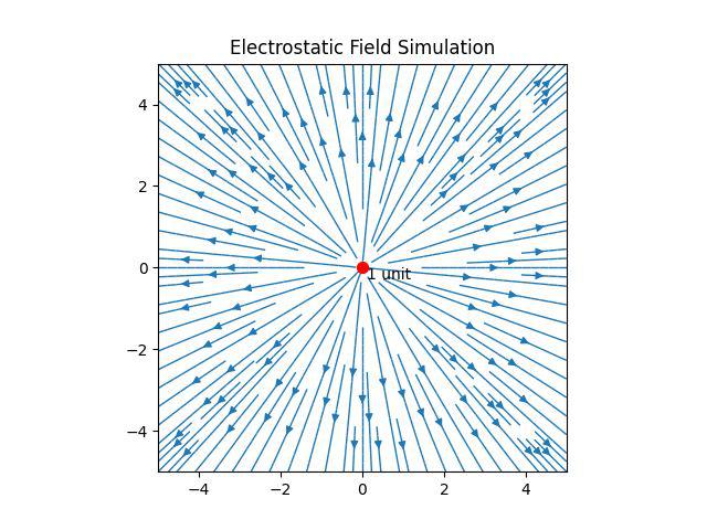
Fig 6: Output of the code

Few more Charge Configurations

Now, you can add or remove any number of charges in the list Q and get equivalent electric field. Here are two example:

Dipole: A dipole is a system of two point charges of equal but opposite magnitudes separated by a distance. Here is the value of Q to get a dipole (of unit magnitude) –

Q = [(-0.5, 0, 1), (0.5, 0, -1)]

Output:

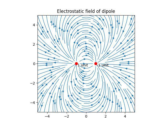
Fig 7: Output of dipole configuration.

Some random charge configuration of multiple charges: As said earlier, you can change Q to any charge configuration. Here is an example

Q = [(0,1,-2), (-2,1,1), (3,-2,3), (0,0,-1), (-4,-4,-5)]

Output

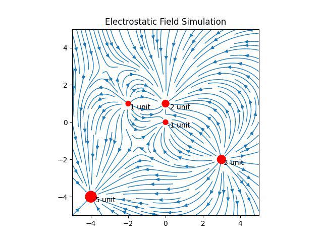
Fig 8: Output of random charges configuration.

Suggest improvement

Three-dimensional Plotting in Python using Matplotlib

Share your thoughts in the comments