In this article, we will learn about sentence autocompletion using TensorFlow. We will follow all the steps that are needed for MLOPs. We will start with importing and cleaning the text, to creating and fitting the model and then we will create a website using Flask framework. In the end, we will deploy the website using Docker. The main goal of this article is to get a brief overview of how MLOPs work and what are the steps.
Dataset for Sentence Autocompletion
We’ve used the Shakespeare Plays dataset which is comprised of plays, characters, lines, and acts in the form of a CSV file.
1. Creating the model for Sentence Autocompletion
Step 1: Importing necessary libraries
Let’s first import all the necessary libraries.
Python3
import re
import numpy as np
import pandas as pd
import numpy as np
import matplotlib.pyplot as plt
import tensorflow as tf
from tensorflow.keras.preprocessing.text import Tokenizer
from tensorflow.keras.preprocessing.sequence import pad_sequences
from tensorflow.keras.layers import Embedding, LSTM, Dense, Dropout
from tensorflow.keras.models import Sequential
from tensorflow.keras.optimizers import Adam
from tensorflow.keras.utils import to_categorical
import pickle
import warnings
warnings.filterwarnings('ignore')
|
Step 2: Loading the dataset
Now, let’s load the dataset and take a look at how the dataset is looking like.
Python3
data = pd.read_csv('Shakespeare_data.csv')
print(data.head())
|
Output:
   Dataline      Play  PlayerLinenumber ActSceneLine         Player  \
0         1  Henry IV               NaN          NaN            NaN
1         2  Henry IV               NaN          NaN            NaN
2         3  Henry IV               NaN          NaN            NaN
3         4  Henry IV               1.0        1.1.1  KING HENRY IV
4         5  Henry IV               1.0        1.1.2  KING HENRY IV
                                          PlayerLine
0                                              ACT I
1                       SCENE I. London. The palace.
2  Enter KING HENRY, LORD JOHN OF LANCASTER, the ...
3             So shaken as we are, so wan with care,
4         Find we a time for frighted peace to pant,
Step 3: Extracting text from the dataset
We want to autocomplete the sentences and thus for that, we will need examples of sentences. We saw from the above dataset that the “PlayerLine” column contained the sentence information. So, let’s extract that column sentence into a text array.
Python3
text = []
for i in data['PlayerLine']:
text.append(i)
text[:5]
|
Output:
['ACT I',
 'SCENE I. London. The palace.',
 'Enter KING HENRY, LORD JOHN OF LANCASTER, the EARL of WESTMORELAND, SIR WALTER BLUNT, and others',
 'So shaken as we are, so wan with care,',
 'Find we a time for frighted peace to pant,']
Step 4: Cleaning Text
Let’s clean the text, this is a very important step as after this step, our sentences will not contain any numbers or any special characters. This will decrease the unnecesary word count that we will generate in the next step.
Python3
def clean_text(text):
pattern = re.compile('[^a-zA-z0-9\s]')
text = re.sub(pattern,'',text)
pattern = re.compile('\d+')
text = re.sub(pattern,'',text)
text = text.lower()
return text
texts = []
for t in text:
new_text = clean_text(t)
texts.append(new_text)
texts[:5]
|
Output:
['act i',
 'scene i london the palace',
 'enter king henry lord john of lancaster the earl of westmoreland sir walter blunt and others',
 'so shaken as we are so wan with care',
 'find we a time for frighted peace to pant']
Step 5: Text vectorization and One hot encoding
1. Text vectorization: Let’s take around 10000 sentences, use the tokenizer from the TensorFlow library and fit it on the sentences. Then let’s generate text sequences i.e. encode the words to numbers. Next, we can pad the sequences up to the maximum sequence length. Here we are using pre-padding so, that 0 will be added before the sentences.
Python3
texts = texts[:10000]
tokenizer = Tokenizer()
tokenizer.fit_on_texts(texts)
text_sequences = np.array(tokenizer.texts_to_sequences(texts))
print('Text -->>',texts[0])
print('Embedding -->>',text_sequences[0])
Max_Sequence_Len = max([len(x) for x in text_sequences])
text_sequences = pad_sequences(text_sequences,
maxlen = Max_Sequence_Len, padding='pre')
print('Maximum Sequence Length -->>',Max_Sequence_Len)
print('Text Sequence -->>\n',text_sequences[0])
print('Text Sequence Shape -->>',text_sequences.shape)
|
Output:
Text -->> act i
Embedding -->> [455, 4]
Maximum Sequence Length -->> 54
Text Sequence -->>
 [  0   0   0   0   0   0   0   0   0   0   0   0   0   0   0   0   0   0
   0   0   0   0   0   0   0   0   0   0   0   0   0   0   0   0   0   0
   0   0   0   0   0   0   0   0   0   0   0   0   0   0   0   0 455   4]
Text Sequence Shape -->> (10000, 54)
2. Splitting the dataset and One hot encoding: Let’s split the dataset into X(input) and y(output). This is many to one-text generation case. Let’s understand the split between the input and output with an example. Assuming the sentence length is n then we will consider n-1 values as input and n^th item as target y.
Our text sequence is pre-padded means to make each sequence of equal length. as per the maximum sequence length which is 54. Here we will put 53 words in X as input, and the last one will be there as y. Hence, we have put every embedded sentence except the last word in X for input and the last word in y. We can see in the shape of X also that it is (10000, 53), which depicts that we have around 53 cols.
Now, as we have only one word in the output so we will have to one hot encode the output. This is done in the following code.
Python3
X, y = text_sequences[:, :-1], text_sequences[:,-1]
print('First Input :',X[0])
print('First Target :',y[0])
word_index = tokenizer.word_index
total_words = len(word_index) + 1
print('Total Number of Words:',total_words)
y = to_categorical(y, num_classes=total_words)
print('Input Shape :',X.shape)
print('Target Shape :',y.shape)
|
Output:
First Input : [  0   0   0   0   0   0   0   0   0   0   0   0   0   0   0   0   0   0
   0   0   0   0   0   0   0   0   0   0   0   0   0   0   0   0   0   0
   0   0   0   0   0   0   0   0   0   0   0   0   0   0   0   0 455]
First Target : 4
Total Number of Words: 7865
Input Shape : (10000, 53)
Target Shape : (10000, 7865)
Step 6: Building the model
Now, let’s build out the LSTM model for the autocompletion of sentences.
- Embedding Layer: We’ll add an embedding layer in which we’ll input the total_words which depicts the size of the data.Next, a vector space of (Max_Sequence_Len – 1) dimensions in which words will be embedded and input sentences have 53 (Max_Sequence_Len – 1, i.e., 54-1) words each.
- LSTM (Long Short Term Memory): Next, we will add the LSTM layer with, here the return_sequences set to be False, hence the layer will only return the last hidden state output.
- Dense Layer: Finally, we’ll add the Dense layer with the softmax activation layer.
- We’ve also added a Dropout layer so as to avoid overfitting.
Let’s see the implementation of the explanation in the following code.
Python3
model = Sequential(name="LSTM_Model")
model.add(Embedding(total_words,
Max_Sequence_Len-1,
input_length=Max_Sequence_Len-1))
model.add(LSTM(512, return_sequences=False))
model.add(Dropout(0.5))
model.add(Dense(total_words, activation='softmax'))
print(model.summary())
|
Output:
Model: "LSTM_Model"
_________________________________________________________________
 Layer (type)                Output Shape              Param #
=================================================================
 embedding (Embedding)       (None, 53, 53)            416845

 lstm (LSTM)                 (None, 512)               1159168

 dropout (Dropout)           (None, 512)               0

 dense (Dense)               (None, 7865)              4034745

=================================================================
Total params: 5,610,758
Trainable params: 5,610,758
Non-trainable params: 0
_________________________________________________________________
None
Step 7: Compiling and Training the Model
For compiling the model, we will use categorical cross-entropy as the labels are one-hot encoded. Next, let’s use Adam optimizer and accuracy as metrics. Then we will train the model for 50 epochs.
Python3
model.compile(
loss="categorical_crossentropy",
optimizer='adam',
metrics=['accuracy']
)
history = model.fit(X, y,
epochs=50,
verbose=1)
|
Output:
Epoch 1/50
313/313 [==============================] - 18s 44ms/step - loss: 7.9333 - accuracy: 0.0114
Epoch 2/50
313/313 [==============================] - 5s 17ms/step - loss: 7.3617 - accuracy: 0.0172
Epoch 3/50
313/313 [==============================] - 5s 16ms/step - loss: 7.1117 - accuracy: 0.0244
Epoch 4/50
313/313 [==============================] - 4s 14ms/step - loss: 6.8334 - accuracy: 0.0297
Epoch 5/50
313/313 [==============================] - 4s 12ms/step - loss: 6.5347 - accuracy: 0.0356
Epoch 6/50
313/313 [==============================] - 4s 14ms/step - loss: 6.2033 - accuracy: 0.0424
Epoch 7/50
313/313 [==============================] - 4s 14ms/step - loss: 5.8106 - accuracy: 0.0550
Epoch 8/50
313/313 [==============================] - 4s 11ms/step - loss: 5.3727 - accuracy: 0.0734
Epoch 9/50
313/313 [==============================] - 4s 13ms/step - loss: 4.8842 - accuracy: 0.0998
Epoch 10/50
313/313 [==============================] - 4s 11ms/step - loss: 4.3616 - accuracy: 0.1479
Epoch 11/50
313/313 [==============================] - 4s 12ms/step - loss: 3.8136 - accuracy: 0.2175
Epoch 12/50
313/313 [==============================] - 4s 13ms/step - loss: 3.2721 - accuracy: 0.3033
Epoch 13/50
313/313 [==============================] - 4s 11ms/step - loss: 2.7658 - accuracy: 0.4034
Epoch 14/50
313/313 [==============================] - 4s 12ms/step - loss: 2.3215 - accuracy: 0.4981
Epoch 15/50
313/313 [==============================] - 4s 12ms/step - loss: 1.9347 - accuracy: 0.5872
Epoch 16/50
313/313 [==============================] - 4s 11ms/step - loss: 1.5971 - accuracy: 0.6602
Epoch 17/50
313/313 [==============================] - 4s 11ms/step - loss: 1.3542 - accuracy: 0.7134
Epoch 18/50
313/313 [==============================] - 4s 13ms/step - loss: 1.1341 - accuracy: 0.7649
Epoch 19/50
313/313 [==============================] - 4s 12ms/step - loss: 0.9632 - accuracy: 0.8013
Epoch 20/50
313/313 [==============================] - 4s 12ms/step - loss: 0.8233 - accuracy: 0.8348
Epoch 21/50
313/313 [==============================] - 4s 11ms/step - loss: 0.7023 - accuracy: 0.8637
Epoch 22/50
313/313 [==============================] - 4s 11ms/step - loss: 0.6235 - accuracy: 0.8786
Epoch 23/50
313/313 [==============================] - 4s 12ms/step - loss: 0.5537 - accuracy: 0.8945
Epoch 24/50
313/313 [==============================] - 4s 13ms/step - loss: 0.5086 - accuracy: 0.8969
Epoch 25/50
313/313 [==============================] - 4s 12ms/step - loss: 0.4629 - accuracy: 0.9075
Epoch 26/50
313/313 [==============================] - 4s 12ms/step - loss: 0.4205 - accuracy: 0.9201
Epoch 27/50
313/313 [==============================] - 4s 12ms/step - loss: 0.3947 - accuracy: 0.9210
Epoch 28/50
313/313 [==============================] - 4s 12ms/step - loss: 0.3685 - accuracy: 0.9276
Epoch 29/50
313/313 [==============================] - 4s 12ms/step - loss: 0.3534 - accuracy: 0.9275
Epoch 30/50
313/313 [==============================] - 4s 12ms/step - loss: 0.3257 - accuracy: 0.9323
Epoch 31/50
313/313 [==============================] - 4s 11ms/step - loss: 0.3175 - accuracy: 0.9317
Epoch 32/50
313/313 [==============================] - 4s 11ms/step - loss: 0.3131 - accuracy: 0.9329
Epoch 33/50
313/313 [==============================] - 4s 12ms/step - loss: 0.2985 - accuracy: 0.9387
Epoch 34/50
313/313 [==============================] - 4s 12ms/step - loss: 0.2844 - accuracy: 0.9385
Epoch 35/50
313/313 [==============================] - 4s 12ms/step - loss: 0.2781 - accuracy: 0.9413
Epoch 36/50
313/313 [==============================] - 4s 11ms/step - loss: 0.2662 - accuracy: 0.9437
Epoch 37/50
313/313 [==============================] - 4s 11ms/step - loss: 0.2526 - accuracy: 0.9441
Epoch 38/50
313/313 [==============================] - 4s 12ms/step - loss: 0.2492 - accuracy: 0.9464
Epoch 39/50
313/313 [==============================] - 4s 11ms/step - loss: 0.2449 - accuracy: 0.9458
Epoch 40/50
313/313 [==============================] - 4s 11ms/step - loss: 0.2426 - accuracy: 0.9467
Epoch 41/50
313/313 [==============================] - 4s 12ms/step - loss: 0.2334 - accuracy: 0.9474
Epoch 42/50
313/313 [==============================] - 4s 11ms/step - loss: 0.2340 - accuracy: 0.9471
Epoch 43/50
313/313 [==============================] - 4s 12ms/step - loss: 0.2344 - accuracy: 0.9472
Epoch 44/50
313/313 [==============================] - 4s 11ms/step - loss: 0.2302 - accuracy: 0.9468
Epoch 45/50
313/313 [==============================] - 4s 12ms/step - loss: 0.2090 - accuracy: 0.9541
Epoch 46/50
313/313 [==============================] - 4s 11ms/step - loss: 0.2077 - accuracy: 0.9525
Epoch 47/50
313/313 [==============================] - 4s 11ms/step - loss: 0.1958 - accuracy: 0.9553
Epoch 48/50
313/313 [==============================] - 4s 11ms/step - loss: 0.2063 - accuracy: 0.9518
Epoch 49/50
313/313 [==============================] - 4s 12ms/step - loss: 0.1970 - accuracy: 0.9547
Epoch 50/50
313/313 [==============================] - 4s 11ms/step - loss: 0.1896 - accuracy: 0.9551
Step 8: Sentence Autocomplete
Now, that our model is trained, let’s auto-complete the sentence using the trained model. Here first used the tokenizer to transform the incomplete sentence into a vector and convert it into the NumPy array. Then we add pre-padding to make the input of max sequence length -1 i.e. 53 in this case. Then we provide this input to the model and get the prediction from the model. The output will be one hot encoded vector. We will get the index of the word from the predicted one hot encoded vector using np.argmax function. Then we will reconvert from index to word from tokenizer.word_index.
Python3
def autoCompletations(text, model):
text_sequences = np.array(tokenizer.texts_to_sequences())
testing = pad_sequences(text_sequences, maxlen = Max_Sequence_Len-1, padding='pre')
y_pred_test = np.argmax(model.predict(testing,verbose=0))
predicted_word = ''
for word, index in tokenizer.word_index.items():
if index == y_pred_test:
predicted_word = word
break
text += " " + predicted_word + '.'
return text
complete_sentence = autoCompletations('I have seen this', model)
complete_sentence
|
Output:
'I have seen this king.'
We can also repeat the above process to add n number of words in our sentence. But it may not give the desired output. Because this is a Many to One model. For this step, we will simply use for loop to get the predicted word from the index using the word_index that was created before.
Python3
def generate_text(text, new_words):
for _ in range(new_words):
text = autoCompletations(text, model)[:-1]
return text
generated_text = generate_text('I have seen', 5)
generated_text
|
Output:
'I have seen lord me death heart king'
Step 9: Saving the model and the tokenizer
Let’s save our model in the form of a .h5 file and also the tokenizer in pickle format. We’ll have to use both of them for the Flask website.
Python3
model.save('sentence_completion.h5')
filename = 'tokenizer.pkl'
pickle.dump(tokenizer, open(filename, 'wb'))
|
2. Creating the Flask website
Step 1: Creating the HTML files
Let’s first create the HTML files, that will work as frontend in our application. We will create the HTML files in the templates folder.
Our first file is index.html. This file contains a form where the user will input the starting text and then the number of words to generate.
HTML
<!DOCTYPE html>
<html>
<head>
<title>Sentence Autocompletion App</title>
</head>
<body>
<form name="form", action = "/generate", method="POST", style="text-align: center;">
<br>
Text: <input type="string" name="Text", placeholder="Enter Text" required/>
<br><br>
No Of Words: <input type="number" name="NoOfWords", placeholder="Enter the no of new words", value="generate" required/>
<br><br>
<button value="Submit">Generate Text</button>
</form>
</body>
</html>
|
Next is generate.html, this will work as an output of the generated text.
HTML
<!DOCTYPE html>
<html>
<head>
<title>Sentence Autocompletion App</title>
</head>
<body>
<form name="form", action = "/generate", method="POST", style="text-align: center;">
<br>
Text: <input type="string" name="Text", placeholder="Enter Text" required/>
<br><br>
No Of Words: <input type="number" name="NoOfWords", placeholder="Enter the no of new words", value="generate" required/>
<br><br>
<button value="Submit">Generate Text</button>
</form>
<p style="text-align: center;">{{ output }}</p>
</body>
</html>
|
Step 2: Creating app.py file
This is the main file, which we will run to run the website. We have simply taken inputs from the forms and then used the model and tokenizer to autocomplete the sentence and then the output will be shown on the website.
Python3
from flask import Flask, render_template, request
import pickle
import numpy as np
from tensorflow.keras.preprocessing.sequence import pad_sequences
import tensorflow as tf
import re
app = Flask(__name__, template_folder='templates')
model = tf.keras.models.load_model('sentence_completion.h5')
with open("tokenizer.pkl", 'rb') as file:
tokenizer = pickle.load(file)
@app.route('/')
def home():
return render_template('index.html')
def autoCompletations(text, model):
text_sequences = np.array(tokenizer.texts_to_sequences())
testing = pad_sequences(text_sequences, maxlen = 53, padding='pre')
y_pred_test = np.argmax(model.predict(testing,verbose=0))
predicted_word = ''
for word, index in tokenizer.word_index.items():
if index == y_pred_test:
predicted_word = word
break
text += " " + predicted_word + '.'
return text
def generate_text(text, new_words):
for _ in range(new_words):
text = autoCompletations(text, model)[:-1]
return text
@app.route('/generate', methods=['GET', 'POST'])
def generate():
if request.method == "POST":
text = request.form.get("Text")
no_of_words = request.form.get("NoOfWords")
generated_text = autoCompletations(text, model)
else:
generated_text = ""
return render_template("generate.html", output = generated_text)
if __name__ == "__main__":
app.run(debug=True)
|
Now, let’s run the project using the following command :
flask run
Step 3: Making a requirements.txt
Let’s create the requirements.txt file using the pip freeze command.
pip freeze > requirements.txt
Step 4: Publishing the code to GitHub
Now, we will have to publish this code to GitHub, for further deployment. For this, you can follow this GitHub article.
3. Step by Step Process for Deploying the project using Docker
For this step, docker must be installed on your machine. You can refer to this article on docker installation.
Checking if the docker is installed on our system or not. For this, you can write the following command on the terminal.
$ docker --version
Now, let’s start the deployment process.
Step 1: Cloning the project
Let’s clone the project on the virtual machine from the GitHub link. For this go to the GitHub repository and copy the link of the GitHub repository. This command will clone the project.
$ git clone https://github.com/<project_name>.git
After this let’s go into the project directory and take a look at the files that are present in the project folder.
$ cd <project_name>
$ ls
Output:
app.py requirement.txt sentence_complete.h5 templates tokenizer.pkl
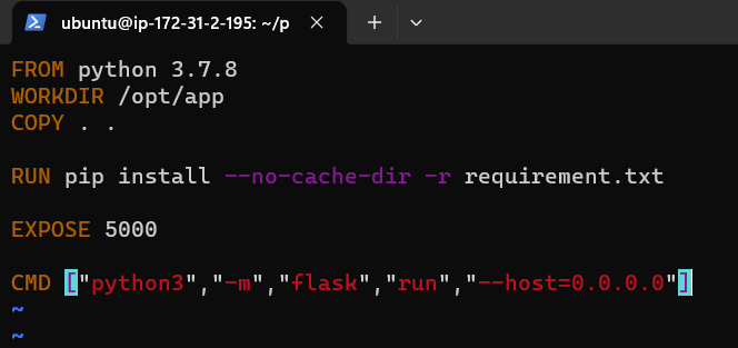
Step 2: Create the Dockerfile
The next step is to create the docker file, for this, we will use the following command:
$ vi Dockerfile
This is how the docker file will look like. For more information on Docker refer to this article on Concepts of Dockerfile, where each step is explained briefly.
Step 3: Building an image by using the docker file
The next step is to build the image, for this, we will use the docker build command. Here ‘:1’ represents the first build.
$ docker build -t username/gfg:1
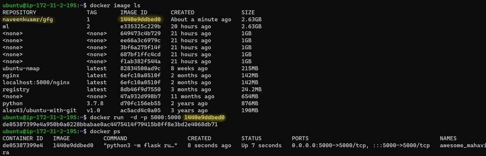
Step 4: Running container
Now, let’s run the container using an image that we have built. For this, we will need the image id, let’s get that from the docker image ls command. The latest build has the image id. Let’s put it in the docker run command.
$ docker image ls
$ docker run -d -p 5000:5000 <image_id>
Step 5: Checking if the container is running or not
Let’s check if the container is running successfully with the following command.
$ docker ps
Step 6: Accessing the website by using the URL from the internet
Now, let’s access the website from the URL on the internet. This is how the website looks like.
Share your thoughts in the comments
Please Login to comment...