PySpark Window Functions

PySpark Window function performs statistical operations such as rank, row number, etc. on a group, frame, or collection of rows and returns results for each row individually. It is also popularly growing to perform data transformations. We will understand the concept of window functions, syntax, and finally how to use them with PySpark SQL and PySpark DataFrame API. 

There are mainly three types of Window function:

• Analytical Function
• Ranking Function
• Aggregate Function

To perform window function operation on a group of rows first, we need to partition i.e. define the group of data rows using window.partition() function, and for row number and rank function we need to additionally order by on partition data using ORDER BY clause. 

Syntax for Window.partition:

Window.partitionBy(“column_name”).orderBy(“column_name”)

Syntax for Window function:

DataFrame.withColumn(“new_col_name”, Window_function().over(Window_partition))

Let’s understand and implement all these functions one by one with examples.

Analytical functions

An analytic function is a function that returns a result after operating on data or a finite set of rows partitioned by a SELECT clause or in the ORDER BY clause. It returns a result in the same number of rows as the number of input rows. E.g. lead(), lag(), cume_dist().

Creating dataframe for demonstration:

Before we start with these functions, first we need to create a DataFrame. We will create a DataFrame that contains employee details like Employee_Name, Age, Department, Salary. After creating the DataFrame we will apply each analytical function on this DataFrame df.

Python3

# importing pyspark
from pyspark.sql.window import Window
import pyspark

# importing sparksession
from pyspark.sql import SparkSession

# creating a sparksession object
# and providing appName
spark = SparkSession.builder.appName("pyspark_window").getOrCreate()

# sample data for dataframe
sampleData = (("Ram", 28, "Sales", 3000),
              ("Meena", 33, "Sales", 4600),
              ("Robin", 40, "Sales", 4100),
              ("Kunal", 25, "Finance", 3000),
              ("Ram", 28, "Sales", 3000),
              ("Srishti", 46, "Management", 3300),
              ("Jeny", 26, "Finance", 3900),
              ("Hitesh", 30, "Marketing", 3000),
              ("Kailash", 29, "Marketing", 2000),
              ("Sharad", 39, "Sales", 4100)
              )

# column names for dataframe
columns = ["Employee_Name", "Age",
           "Department", "Salary"]

# creating the dataframe df
df = spark.createDataFrame(data=sampleData,
                           schema=columns)

# importing Window from pyspark.sql.window

# creating a window
# partition of dataframe
windowPartition = Window.partitionBy("Department").orderBy("Age")

# print schema
df.printSchema()

# show df
df.show()

Output:

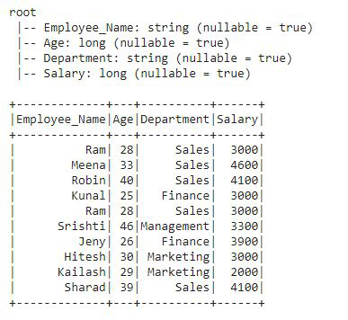
This is the DataFrame on which we will apply all the analytical functions.

Example 1: Using cume_dist()

cume_dist() window function is used to get the cumulative distribution within a window partition. It is similar to CUME_DIST in SQL. Let’s see an example:

Python3

# importing cume_dist()
# from pyspark.sql.functions
from pyspark.sql.functions import cume_dist

# applying window function with
# the help of DataFrame.withColumn
df.withColumn("cume_dist",
              cume_dist().over(windowPartition)).show()

Output:

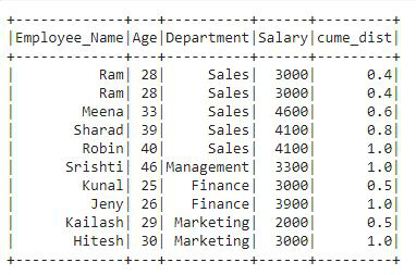
In the output, we can see that a new column is added to the df named “cume_dist” that contains the cumulative distribution of the Department column which is ordered by the Age column.

Example 2: Using lag()

A lag() function is used to access previous rows’ data as per the defined offset value in the function. This function is similar to the LAG in SQL.

Python3

# importing lag() from pyspark.sql.functions
from pyspark.sql.functions import lag

df.withColumn("Lag", lag("Salary", 2).over(windowPartition)) \
    .show()

Output:

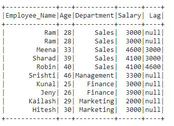
In the output, we can see that lag column is added to the df that contains lag values. In the first 2 rows there is a null value as we have defined offset 2 followed by column Salary in the lag() function. The next rows contain the values of previous rows.

Example 3: Using lead()

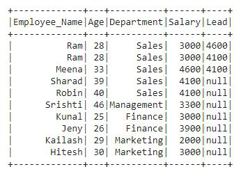
A lead() function is used to access next rows data as per the defined offset value in the function. This function is similar to the LEAD in SQL and just opposite to lag() function or LAG in SQL.

Python3

# importing lead() from pyspark.sql.functions
from pyspark.sql.functions import lead

df.withColumn("Lead", lead("salary", 2).over(windowPartition)) \
    .show()

Output:

Ranking Function

The function returns the statistical rank of a given value for each row in a partition or group. The goal of this function is to provide consecutive numbering of the rows in the resultant column, set by the order selected in the Window.partition for each partition specified in the OVER clause. E.g. row_number(), rank(), dense_rank(), etc.

Creating Dataframe for demonstration:

Before we start with these functions, first we need to create a DataFrame. We will create a DataFrame that contains student details like Roll_No, Student_Name, Subject, Marks. After creating the DataFrame we will apply each Ranking function on this DataFrame df2.

Python3

# importing pyspark
from pyspark.sql.window import Window
import pyspark

# importing sparksession
from pyspark.sql import SparkSession

# creating a sparksession object and providing appName
spark = SparkSession.builder.appName("pyspark_window").getOrCreate()

# sample data for dataframe
sampleData = ((101, "Ram", "Biology", 80),
              (103, "Meena", "Social Science", 78),
              (104, "Robin", "Sanskrit", 58),
              (102, "Kunal", "Phisycs", 89),
              (101, "Ram", "Biology", 80),
              (106, "Srishti", "Maths", 70),
              (108, "Jeny", "Physics", 75),
              (107, "Hitesh", "Maths", 88),
              (109, "Kailash", "Maths", 90),
              (105, "Sharad", "Social Science", 84)
              )

# column names for dataframe
columns = ["Roll_No", "Student_Name", "Subject", "Marks"]

# creating the dataframe df
df2 = spark.createDataFrame(data=sampleData,
                            schema=columns)

# importing window from pyspark.sql.window

# creating a window partition of dataframe
windowPartition = Window.partitionBy("Subject").orderBy("Marks")

# print schema
df2.printSchema()

# show df
df2.show()

Output:

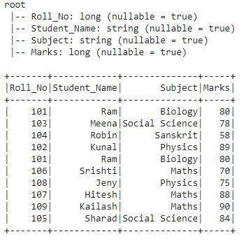
This is the DataFrame df2 on which we will apply all the Window ranking function.

Example 1: Using row_number().

row_number() function is used to gives a sequential number to each row present in the table. Let’s see the example:

Python3

# importing row_number() from pyspark.sql.functions
from pyspark.sql.functions import row_number

# applying the row_number() function
df2.withColumn("row_number",
               row_number().over(windowPartition)).show()

Output:

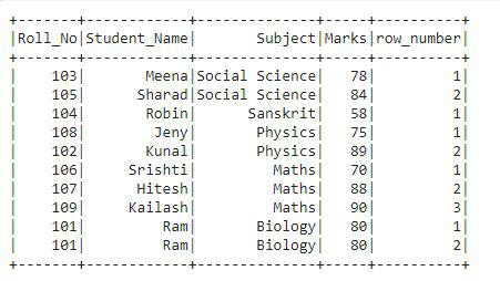
In this output, we can see that we have the row number for each row based on the specified partition i.e. the row numbers are given followed by the Subject and Marks column. 

Example 2: Using rank()

The rank function is used to give ranks to rows specified in the window partition. This function leaves gaps in rank if there are ties. Let’s see the example:

Python3

# importing rank() from pyspark.sql.functions
from pyspark.sql.functions import rank

# applying the rank() function
df2.withColumn("rank", rank().over(windowPartition)) \
    .show()

Output:

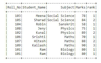
In the output, the rank is provided to each row as per the Subject and Marks column as specified in the window partition.

Example 3: Using percent_rank()

This function is similar to rank() function. It also provides rank to rows but in a percentile format. Let’s see the example: 

Python3

# importing percent_rank() from pyspark.sql.functions
from pyspark.sql.functions import percent_rank

# applying the percent_rank() function
df2.withColumn("percent_rank",
               percent_rank().over(windowPartition)).show()

Output:

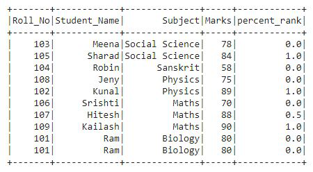
We can see that in the output the rank column contains values in a percentile form i.e. in the decimal format.

Example 4: Using dense_rank()

This function is used to get the rank of each row in the form of row numbers. This is similar to rank() function, there is only one difference the rank function leaves gaps in rank when there are ties. Let’s see the example:

Python3

# importing dense_rank() from pyspark.sql.functions
from pyspark.sql.functions import dense_rank

# applying the dense_rank() function
df2.withColumn("dense_rank",
               dense_rank().over(windowPartition)).show()

Output:

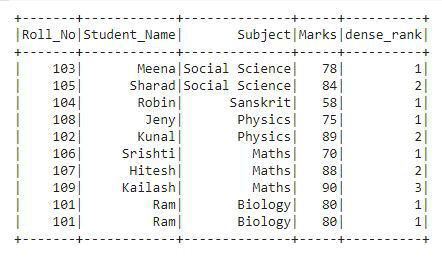
In the output, we can see that the ranks are given in the form of row numbers. 

Aggregate function

An aggregate function or aggregation function is a function where the values of multiple rows are grouped to form a single summary value. The definition of the groups of rows on which they operate is done by using the SQL GROUP BY clause. E.g. AVERAGE, SUM, MIN, MAX, etc. 

Creating Dataframe for demonstration:

Before we start with these functions, we will create a new DataFrame that contains employee details like Employee_Name, Department, and Salary. After creating the DataFrame we will apply each Aggregate function on this DataFrame.

Python3

# importing pyspark
import pyspark

# importing sparksessio
from pyspark.sql import SparkSession

# creating a sparksession
# object and providing appName
spark = SparkSession.builder.appName("pyspark_window").getOrCreate()

# sample data for dataframe
sampleData = (("Ram", "Sales", 3000),
              ("Meena", "Sales", 4600),
              ("Robin", "Sales", 4100),
              ("Kunal", "Finance", 3000),
              ("Ram", "Sales", 3000),
              ("Srishti", "Management", 3300),
              ("Jeny", "Finance", 3900),
              ("Hitesh", "Marketing", 3000),
              ("Kailash", "Marketing", 2000),
              ("Sharad", "Sales", 4100)
              )

# column names for dataframe
columns = ["Employee_Name", "Department", "Salary"]

# creating the dataframe df
df3 = spark.createDataFrame(data=sampleData,
                            schema=columns)

# print schema
df3.printSchema()

# show df
df3.show()

Output:

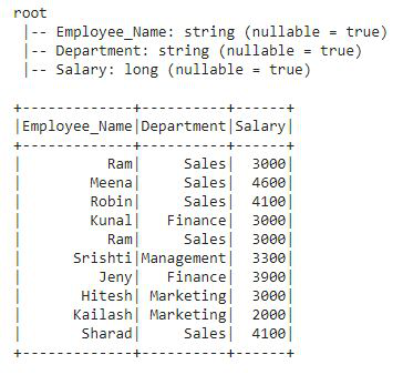
This is the DataFrame df3 on which we will apply all the aggregate functions.

Example: Let’s see how to apply the aggregate functions with this example

Python3

# importing window from pyspark.sql.window
from pyspark.sql.window import Window

# importing aggregate functions
# from pyspark.sql.functions
from pyspark.sql.functions import col,avg,sum,min,max,row_number

# creating a window partition of dataframe
windowPartitionAgg  = Window.partitionBy("Department")

# applying window aggregate function
# to df3 with the help of withColumn

# this is average()
df3.withColumn("Avg",
               avg(col("salary")).over(windowPartitionAgg))
    #this is sum()
  .withColumn("Sum",
              sum(col("salary")).over(windowPartitionAgg))
    #this is min()
  .withColumn("Min",
              min(col("salary")).over(windowPartitionAgg))
    #this is max()
  .withColumn("Max",
              max(col("salary")).over(windowPartitionAgg)).show()

Output:

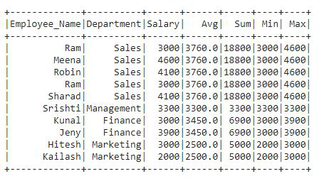
In the output df, we can see that there are four new columns added to df.  In the code, we have applied all the four aggregate functions one by one. We got four output columns added to the df3 that contains values for each row. These four columns contain the Average, Sum, Minimum, and Maximum values of the Salary column.