Within the intricate landscape of semantic segmentation, the Pyramid Scene Parsing Network or PSPNet has emerged as a formidable architecture by showcasing unparalleled performance in deciphering intricate scenes. In this article, we will discuss about PSPNet and implement it.
What is Semantic Segmentation?
Semantic segmentation stands as a cutting-edge technique in computer vision, crucial for unraveling and deciphering the visual content embedded in images. Unlike the traditional approach of assigning a single label to an entire image, semantic segmentation dives deeper by meticulously categorizing each pixel, essentially creating a pixel-level map of distinct classes or objects. The objective is to intricately divide an image into coherent segments, linking each pixel to a specific object or region. This granular approach empowers computers to grasp intricate details and spatial relationships within a scene, fostering a nuanced comprehension of visual information. The versatility of semantic segmentation extends across varied domains like autonomous driving, medical imaging, and augmented reality, where pinpoint accuracy in delineating objects and their boundaries is imperative for precise decision-making and comprehensive analysis. By delivering a meticulous understanding of images, semantic segmentation serves as the cornerstone for an array of advanced computer vision tasks and applications.
What is PSPNet?
PSPNet, an acronym for Pyramid Scene Parsing Network, constitutes a profound Deep Learning model meticulously crafted for pixel-wise semantic segmentation of images. Developed by Heng Shuang Zhao et al. in 2017, PSPNet adeptly tackles the challenges associated with capturing contextual information across diverse scales within an image. The architecture is accomplished through the integration of a pioneering pyramid pooling module, empowering the network to encapsulate intricate contextual details and elevate segmentation precision.
Some of the key-working principals of PSPNet is discussed below:
- Pyramid Pooling Module: The crux of its innovation lies in its pyramid pooling module which is specially designed to encapsulate multi-scale contextual information. By partitioning the input feature map into distinct regions and applying adaptive pooling across various scales, it ensures the network’s adeptness in scrutinizing both nuanced intricacies and broader contextual nuances.
- Residual Blocks with Dilated Convolutions: PSPNet strategically employs residual blocks featuring dilated convolutions to distill features from input images. The utilization of dilated convolutions facilitates an expanded receptive field without a surge in parameters, thus accommodating the assimilation of more extensive contextual information. This augmentation significantly contributes to the model’s prowess in comprehending complex scenes and refining segmentation accuracy.
- Image Pyramid: PSPNet harnesses the potential of an image pyramid to process input images at multiple resolutions. This strategic approach empowers the network to analyze images across varying scales, capturing the intricacies of both local and global contexts. The synergistic interplay between the pyramid pooling module and the image pyramid propels it’s proficiency in segmenting objects of diverse sizes and characteristics.
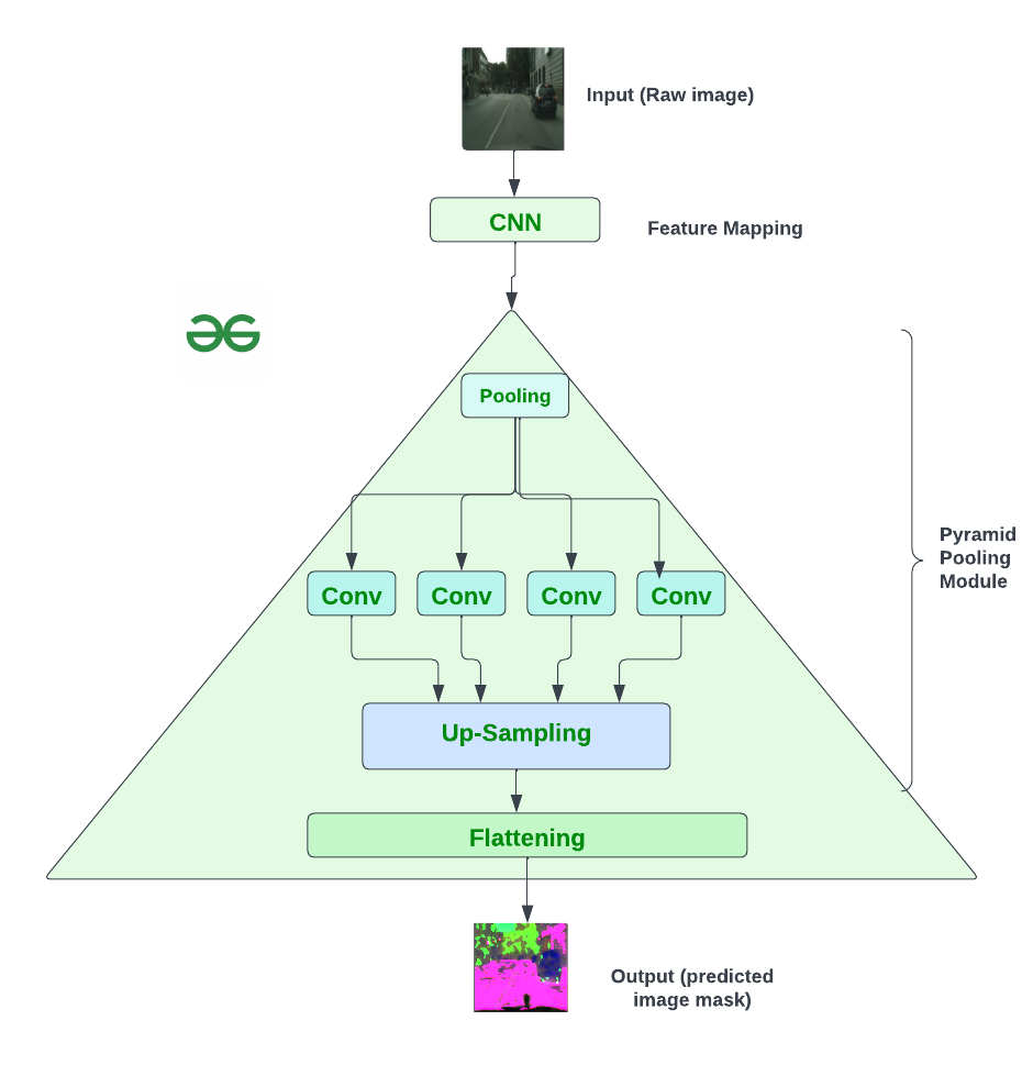
Architecture of the PSPNet
Architecture of PSPNet is little complex which is discussed below:
- Input and Feature Extraction
- The process begins with an input image, which undergoes feature extraction using a pretrained ResNet model with a dilated network strategy.
- The dilated network strategy helps extract detailed information from the image, and the final feature map size is 1/8 of the input image.
- Pyramid Pooling Module
- The Pyramid Pooling Module is introduced to gather contextual information on top of the extracted feature map.
- A 4-level pyramid is created, covering the entire image, half of the image, and small portions. These levels serve as a global prior for understanding the scene.
- The pooling kernels at different levels capture various contextual scales.
- The information from the pyramid is fused as the global prior and concatenated with the original feature map from the ResNet model.
- Final Prediction
- The concatenated information is then processed through a convolutional layer to generate the final prediction map.
- The convolutional layer refines the combined information, providing a detailed prediction of pixel-level scene parsing.
In short, the architecture leverages a pretrained model named ResNet with a dilated network strategy for feature extraction, enhances contextual understanding through Pyramid Pooling Module and efficiently generates pixel-level scene predictions.
Pyramid Pooling Module
The Pyramid Pooling Module (PPM) is a crucial component in the architecture of PSPNet, designed to capture global contextual information effectively. It operates at multiple scales, fusing features from different sub-regions, and provides an effective global contextual prior for pixel-level scene parsing in the PSPNet architecture.
Pyramid Pooling Operation
- The Pyramid Pooling Module fuses features under four different pyramid scales (1×1, 2×2, 3×3, and 6×6).
- The coarsest level (highlighted in red) involves global pooling, generating a single bin output.
- Subsequent levels separate the feature map into different sub-regions and form pooled representations for different locations.
- Each pyramid level’s dimension is reduced using 1×1 convolution layers to maintain the weight of global features.
- Low-dimensional feature maps are upsampled via bilinear interpolation to match the original feature map size.
- Finally, different levels of features are concatenated to form the final pyramid pooling global feature.
PSPNet model Architecture
Step-by-step implementation
Importing required libraries
At first, we will import all required Python libraries like NumPy, TensorFlow, Matplotlib, OS etc.
Python3
import numpy as np
import time
import os
import matplotlib.pyplot as plt
import cv2
import tensorflow as tf
from tensorflow import keras
import tensorflow.keras.backend as K
from tensorflow.keras.layers import Convolution2D, BatchNormalization, ReLU, LeakyReLU, Add, Activation
from tensorflow.keras.layers import GlobalAveragePooling2D, AveragePooling2D, UpSampling2D
|
Dataset loading and pre-processing
You can download the dataset from here. After that, we will define a small function (load_image_mask_subset) to extract the image masks as segments to implement PSPNet further. Here we will load a small subset of dataset as per machine capabilities (Without GPU, average standard RAM) but it is recommended to use more subsamples or full dataset for better model performance.
Python3
num_train_samples = 50
num_valid_samples = 10
def load_image_mask_subset(path, num_samples=None):
file_names = os.listdir(path)[:num_samples]
image_list, mask_list = [], []
for file_name in file_names:
image = cv2.imread(os.path.join(path, file_name))
image = cv2.normalize(image, None, 0, 1, cv2.NORM_MINMAX, cv2.CV_32F)
image = image[:, :, ::-1]
image_list.append(image[:, :256])
mask_list.append(np.reshape(image[:, 256:], (256 * 256 * 3)))
del image
del file_names
return image_list, mask_list
train_data_folder = "/content/cityscapes-image-pairs/cityscapes_data/train/"
valid_data_folder = "/content/cityscapes-image-pairs/cityscapes_data/val/"
train_images, train_masks = load_image_mask_subset(train_data_folder, num_samples=num_train_samples)
valid_images, valid_masks = load_image_mask_subset(valid_data_folder, num_samples=num_valid_samples)
|
Defining PSPNet model
PSPNet model is a multilayered model and requires multiple definition of each block with careful attention and loss reduction.
- Convolutional blocks: We will define a building block commonly used in advanced image recognition systems, particularly those designed for tasks like understanding scenes in images. Think of it as a mini-processor that takes in visual information and processes it in three distinct steps, each represented by ‘block_a’, ‘block_b’, and ‘block_c’. In these steps, it applies different filters and transformations to capture various aspects of the input. Importantly, it incorporates a smart shortcut, allowing the original information to bypass some of the processing. This technique, known as skip connection or residual connection, helps the network learn more effectively. It’s akin to having a main road (original input) and a shortcut (skip connection) to efficiently navigate through the processing steps. Finally, it produces a refined output that can be more informative for understanding complex visual patterns.
Python3
def convolutional_block(input_tensor, filters, block_identifier):
block_name = 'block_' + str(block_identifier) + '_'
filter1, filter2, filter3 = filters
skip_connection = input_tensor
input_tensor = Convolution2D(filters=filter1, kernel_size=(1, 1), dilation_rate=(1, 1),
padding='same', kernel_initializer='he_normal', name=block_name + 'a')(input_tensor)
input_tensor = BatchNormalization(name=block_name + 'batch_norm_a')(input_tensor)
input_tensor = LeakyReLU(alpha=0.2, name=block_name + 'leakyrelu_a')(input_tensor)
input_tensor = Convolution2D(filters=filter2, kernel_size=(3, 3), dilation_rate=(2, 2),
padding='same', kernel_initializer='he_normal', name=block_name + 'b')(input_tensor)
input_tensor = BatchNormalization(name=block_name + 'batch_norm_b')(input_tensor)
input_tensor = LeakyReLU(alpha=0.2, name=block_name + 'leakyrelu_b')(input_tensor)
input_tensor = Convolution2D(filters=filter3, kernel_size=(1, 1), dilation_rate=(1, 1),
padding='same', kernel_initializer='he_normal', name=block_name + 'c')(input_tensor)
input_tensor = BatchNormalization(name=block_name + 'batch_norm_c')(input_tensor)
skip_connection = Convolution2D(filters=filter3, kernel_size=(3, 3), padding='same', name=block_name + 'skip_conv')(skip_connection)
skip_connection = BatchNormalization(name=block_name + 'batch_norm_skip_conv')(skip_connection)
input_tensor = Add(name=block_name + 'add')([input_tensor, skip_connection])
input_tensor = ReLU(name=block_name + 'relu')(input_tensor)
return input_tensor
|
- Feature mapping: In the middle of the pyramid we will define two essential components in a sophisticated image analysis system. First, the
base_convolutional_block function serves as a foundational block for extracting essential features from an input image. It does this by applying a series of convolutional operations, organized into three separate blocks labeled ‘base block 1’, ‘base block 2’, and ‘base block 3’. Each block progressively refines and abstracts the visual information, employing a clever skip connection strategy to retain crucial details from the original input. Building upon the base feature extraction, the pyramid_pooling_module function introduces a unique module known as the pyramid pooling module. This module strategically pools information from different pixels to capture diverse contextual details. It starts with the base feature maps obtained from the base_convolutional_block function. The module then performs pixel pooling operations, aptly named ‘red pixel pooling’, ‘yellow pixel pooling’, ‘blue pixel pooling’, and ‘green pixel pooling’. These operations extract valuable information at various resolutions, and the resulting pixel pools are then intelligently combined into a final pyramid pooling. This comprehensive pooling process ensures that the model gains a holistic understanding of the image, considering both fine details and broader contextual information.
Python3
def base_convolutional_block(input_layer):
base_result = convolutional_block(input_layer, [32, 32, 64], '1')
base_result = convolutional_block(base_result, [64, 64, 128], '2')
base_result = convolutional_block(base_result, [128, 128, 256], '3')
return base_result
def pyramid_pooling_module(input_layer):
base_result = base_convolutional_block(input_layer)
red_result = GlobalAveragePooling2D(name='red_pool')(base_result)
red_result = tf.keras.layers.Reshape((1, 1, 256))(red_result)
red_result = Convolution2D(filters=64, kernel_size=(1, 1), name='red_1_by_1')(red_result)
red_result = UpSampling2D(size=256, interpolation='bilinear', name='red_upsampling')(red_result)
yellow_result = AveragePooling2D(pool_size=(2, 2), name='yellow_pool')(base_result)
yellow_result = Convolution2D(filters=64, kernel_size=(1, 1), name='yellow_1_by_1')(yellow_result)
yellow_result = UpSampling2D(size=2, interpolation='bilinear', name='yellow_upsampling')(yellow_result)
blue_result = AveragePooling2D(pool_size=(4, 4), name='blue_pool')(base_result)
blue_result = Convolution2D(filters=64, kernel_size=(1, 1), name='blue_1_by_1')(blue_result)
blue_result = UpSampling2D(size=4, interpolation='bilinear', name='blue_upsampling')(blue_result)
green_result = AveragePooling2D(pool_size=(8, 8), name='green_pool')(base_result)
green_result = Convolution2D(filters=64, kernel_size=(1, 1), name='green_1_by_1')(green_result)
green_result = UpSampling2D(size=8, interpolation='bilinear', name='green_upsampling')(green_result)
return tf.keras.layers.concatenate([base_result, red_result, yellow_result, blue_result, green_result])
|
- Base of the Pyramid: In this last block of pyramid, the
pyramid_based_conv function orchestrates the final stages of our PSPNet model. It takes as input the feature maps obtained from the previous processing stages, specifically from the pyramid_pooling_module function. The essence of this module is to distill the intricate hierarchical representations learned by the model into a more compact and interpretable output. It employs a convolutional layer, denoted as ‘last convolution 3 by 3’, which refines the features spatially. Batch normalization is applied to ensure stable and efficient training, followed by a sigmoid activation function to produce pixel-wise predictions. This activation function scales the output values between 0 and 1, effectively transforming them into probabilities. Lastly, the output is flattened to create a one-dimensional representation, encapsulating the model’s final insights into the input image.
Python3
def pyramid_based_conv(input_layer):
result = pyramid_pooling_module(input_layer)
result = Convolution2D(filters=3, kernel_size=3, padding='same', name='last_conv_3_by_3')(result)
result = BatchNormalization(name='last_conv_3_by_3_batch_norm')(result)
result = Activation('sigmoid', name='last_conv_relu')(result)
result = tf.keras.layers.Flatten(name='last_conv_flatten')(result)
return result
input_layer = tf.keras.Input(shape=np.squeeze(train_images[0]).shape, name='input')
output_layer = pyramid_based_conv(input_layer)
|
Visualizing the model
We have already defined the whole PSPNet model. Let’s have a look of it for better understanding.
Python3
model = tf.keras.Model(inputs=input_layer,outputs=output_layer)
model.summary()
|
Output:
Model: "model"
__________________________________________________________________________________________________
 Layer (type)                Output Shape                 Param #   Connected to
==================================================================================================
 input (InputLayer)          [(None, 256, 256, 3)]        0         []

 block_1_a (Conv2D)          (None, 256, 256, 32)         128       ['input[0][0]']

 block_1_batch_norm_a (Batc  (None, 256, 256, 32)         128       ['block_1_a[0][0]']
 hNormalization)

 block_1_leakyrelu_a (Leaky  (None, 256, 256, 32)         0         ['block_1_batch_norm_a[0][0]']
 ReLU)

 block_1_b (Conv2D)          (None, 256, 256, 32)         9248      ['block_1_leakyrelu_a[0][0]']

 block_1_batch_norm_b (Batc  (None, 256, 256, 32)         128       ['block_1_b[0][0]']
 hNormalization)

 block_1_leakyrelu_b (Leaky  (None, 256, 256, 32)         0         ['block_1_batch_norm_b[0][0]']
 ReLU)

 block_1_c (Conv2D)          (None, 256, 256, 64)         2112      ['block_1_leakyrelu_b[0][0]']

 block_1_skip_conv (Conv2D)  (None, 256, 256, 64)         1792      ['input[0][0]']

 block_1_batch_norm_c (Batc  (None, 256, 256, 64)         256       ['block_1_c[0][0]']
 hNormalization)

 block_1_batch_norm_skip_co  (None, 256, 256, 64)         256       ['block_1_skip_conv[0][0]']
 nv (BatchNormalization)

 block_1_add (Add)           (None, 256, 256, 64)         0         ['block_1_batch_norm_c[0][0]',
                                                                     'block_1_batch_norm_skip_conv
                                                                    [0][0]']

 block_1_relu (ReLU)         (None, 256, 256, 64)         0         ['block_1_add[0][0]']

 block_2_a (Conv2D)          (None, 256, 256, 64)         4160      ['block_1_relu[0][0]']

 block_2_batch_norm_a (Batc  (None, 256, 256, 64)         256       ['block_2_a[0][0]']
 hNormalization)

 block_2_leakyrelu_a (Leaky  (None, 256, 256, 64)         0         ['block_2_batch_norm_a[0][0]']
 ReLU)

 block_2_b (Conv2D)          (None, 256, 256, 64)         36928     ['block_2_leakyrelu_a[0][0]']

 block_2_batch_norm_b (Batc  (None, 256, 256, 64)         256       ['block_2_b[0][0]']
 hNormalization)

 block_2_leakyrelu_b (Leaky  (None, 256, 256, 64)         0         ['block_2_batch_norm_b[0][0]']
 ReLU)

 block_2_c (Conv2D)          (None, 256, 256, 128)        8320      ['block_2_leakyrelu_b[0][0]']

 block_2_skip_conv (Conv2D)  (None, 256, 256, 128)        73856     ['block_1_relu[0][0]']

 block_2_batch_norm_c (Batc  (None, 256, 256, 128)        512       ['block_2_c[0][0]']
 hNormalization)

 block_2_batch_norm_skip_co  (None, 256, 256, 128)        512       ['block_2_skip_conv[0][0]']
 nv (BatchNormalization)

 block_2_add (Add)           (None, 256, 256, 128)        0         ['block_2_batch_norm_c[0][0]',
                                                                     'block_2_batch_norm_skip_conv
                                                                    [0][0]']

 block_2_relu (ReLU)         (None, 256, 256, 128)        0         ['block_2_add[0][0]']

 block_3_a (Conv2D)          (None, 256, 256, 128)        16512     ['block_2_relu[0][0]']

 block_3_batch_norm_a (Batc  (None, 256, 256, 128)        512       ['block_3_a[0][0]']
 hNormalization)

 block_3_leakyrelu_a (Leaky  (None, 256, 256, 128)        0         ['block_3_batch_norm_a[0][0]']
 ReLU)

 block_3_b (Conv2D)          (None, 256, 256, 128)        147584    ['block_3_leakyrelu_a[0][0]']

 block_3_batch_norm_b (Batc  (None, 256, 256, 128)        512       ['block_3_b[0][0]']
 hNormalization)

 block_3_leakyrelu_b (Leaky  (None, 256, 256, 128)        0         ['block_3_batch_norm_b[0][0]']
 ReLU)

 block_3_c (Conv2D)          (None, 256, 256, 256)        33024     ['block_3_leakyrelu_b[0][0]']

 block_3_skip_conv (Conv2D)  (None, 256, 256, 256)        295168    ['block_2_relu[0][0]']

 block_3_batch_norm_c (Batc  (None, 256, 256, 256)        1024      ['block_3_c[0][0]']
 hNormalization)

 block_3_batch_norm_skip_co  (None, 256, 256, 256)        1024      ['block_3_skip_conv[0][0]']
 nv (BatchNormalization)

 block_3_add (Add)           (None, 256, 256, 256)        0         ['block_3_batch_norm_c[0][0]',
                                                                     'block_3_batch_norm_skip_conv
                                                                    [0][0]']

 block_3_relu (ReLU)         (None, 256, 256, 256)        0         ['block_3_add[0][0]']

 red_pool (GlobalAveragePoo  (None, 256)                  0         ['block_3_relu[0][0]']
 ling2D)

 reshape (Reshape)           (None, 1, 1, 256)            0         ['red_pool[0][0]']

 yellow_pool (AveragePoolin  (None, 128, 128, 256)        0         ['block_3_relu[0][0]']
 g2D)

 blue_pool (AveragePooling2  (None, 64, 64, 256)          0         ['block_3_relu[0][0]']
 D)

 green_pool (AveragePooling  (None, 32, 32, 256)          0         ['block_3_relu[0][0]']
 2D)

 red_1_by_1 (Conv2D)         (None, 1, 1, 64)             16448     ['reshape[0][0]']

 yellow_1_by_1 (Conv2D)      (None, 128, 128, 64)         16448     ['yellow_pool[0][0]']

 blue_1_by_1 (Conv2D)        (None, 64, 64, 64)           16448     ['blue_pool[0][0]']

 green_1_by_1 (Conv2D)       (None, 32, 32, 64)           16448     ['green_pool[0][0]']

 red_upsampling (UpSampling  (None, 256, 256, 64)         0         ['red_1_by_1[0][0]']
 2D)

 yellow_upsampling (UpSampl  (None, 256, 256, 64)         0         ['yellow_1_by_1[0][0]']
 ing2D)

 blue_upsampling (UpSamplin  (None, 256, 256, 64)         0         ['blue_1_by_1[0][0]']
 g2D)

 green_upsampling (UpSampli  (None, 256, 256, 64)         0         ['green_1_by_1[0][0]']
 ng2D)

 concatenate (Concatenate)   (None, 256, 256, 512)        0         ['block_3_relu[0][0]',
                                                                     'red_upsampling[0][0]',
                                                                     'yellow_upsampling[0][0]',
                                                                     'blue_upsampling[0][0]',
                                                                     'green_upsampling[0][0]']

 last_conv_3_by_3 (Conv2D)   (None, 256, 256, 3)          13827     ['concatenate[0][0]']

 last_conv_3_by_3_batch_nor  (None, 256, 256, 3)          12        ['last_conv_3_by_3[0][0]']
 m (BatchNormalization)

 last_conv_relu (Activation  (None, 256, 256, 3)          0         ['last_conv_3_by_3_batch_norm[
 )                                                                  0][0]']

 last_conv_flatten (Flatten  (None, 196608)               0         ['last_conv_relu[0][0]']
 )

==================================================================================================
Total params: 713839 (2.72 MB)
Trainable params: 711145 (2.71 MB)
Non-trainable params: 2694 (10.52 KB)
__________________________________________________________________________________________________
Model training
Now we will train the PSPNet model on 10 epochs, batch size 8, learning rate 0.001 with loss function as MSE and optimizer Adam.
Python3
model.compile(optimizer=tf.keras.optimizers.Adam(learning_rate=0.001),loss='mse')
history = model.fit(np.array(train_images,dtype='float16'),np.array(train_masks,dtype='float16'),
validation_data=(np.array(valid_images,dtype='float16'),np.array(valid_masks,dtype='float16')),
epochs=10,steps_per_epoch=5,verbose=1,batch_size=8)
|
Output:
Epoch 1/10
5/5 [==============================] - 41s 2s/step - loss: 0.0413 - val_loss: 0.1369
Epoch 2/10
5/5 [==============================] - 10s 2s/step - loss: 0.0394 - val_loss: 0.1508
Epoch 3/10
5/5 [==============================] - 4s 797ms/step - loss: 0.0455 - val_loss: 0.1332
Epoch 4/10
5/5 [==============================] - 5s 977ms/step - loss: 0.0390 - val_loss: 0.1469
Epoch 5/10
5/5 [==============================] - 4s 965ms/step - loss: 0.0374 - val_loss: 0.1382
Epoch 6/10
5/5 [==============================] - 4s 867ms/step - loss: 0.0369 - val_loss: 0.1298
Epoch 7/10
5/5 [==============================] - 4s 800ms/step - loss: 0.0408 - val_loss: 0.1270
Epoch 8/10
5/5 [==============================] - 5s 963ms/step - loss: 0.0364 - val_loss: 0.1259
Epoch 9/10
5/5 [==============================] - 4s 802ms/step - loss: 0.0369 - val_loss: 0.1385
Epoch 10/10
5/5 [==============================] - 4s 800ms/step - loss: 0.0365 - val_loss: 0.1409
Visualizing model performance
Now we will plot training and validation loss to understand the model’s training progress.
Python3
plt.figure(figsize=(10, 4))
plt.subplot(1, 2, 1)
plt.plot(history.history['loss'], label='Training Loss')
plt.plot(history.history['val_loss'], label='Validation Loss')
plt.title('Training vs. Validation Loss')
plt.xlabel('Epochs')
plt.ylabel('Loss')
plt.legend()
plt.show()
|
Output:
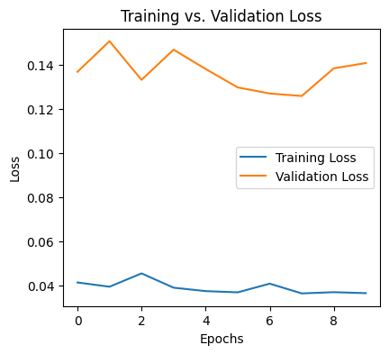
Training vs. validation loss
From the output it is very clear that we must go for more epochs to get a better model if we have sufficient machine resources.
Visualizing predictions
As PSPNet is a segmentation model so there are no good metrics to evaluate it logically. But we can evaluation it’s performance based on visualizing predicted masks with comparison to actual mask. We will randomly make comparison by taking one image from validation set and plot it for comparison. Note that we have trained our model with less data and less number of epochs. So, output may not be cleared but we can check if attention line (object wise color difference line) is visible or not.
Python3
def plot_imgs(img,mask,pred):
mask = np.reshape(mask,(256,256,3))
pred = np.reshape(pred,(256,256,3))
fig,(ax1,ax2,ax3) = plt.subplots(1,3,figsize=(15,10))
ax1.imshow(img)
ax1.axis('off')
ax2.imshow(mask)
ax2.axis('off')
ax3.imshow(pred)
ax3.axis('off')
pred_masks = model.predict(np.array(valid_images,dtype='float16'))
print('-------------Input---------------Actual mask--------------Predicted mask-------')
for i in range(1):
x = np.random.randint(0,10,size=1)[0]
plot_imgs(valid_images[x],valid_masks[x],pred_masks[x])
|
Output:
1/1 [==============================] - 0s 344ms/step
-------------Input---------------Actual mask--------------Predicted mask-------
.png)
Comparative output plot
From the above output we can see that the predicted mask is not clear because model is trained on less data and less number of epochs. However, the attention lines are clearly placed by the model. So, we can continue will this model to perform model training epochs on large data.
Share your thoughts in the comments
Please Login to comment...