Power Spectral Density

In terms of electronics, Power is defined as the total amount of energy that is getting transferred or converted per unit measurement of time, or in general terms Power is defined as the strength or the intensity level of the signal. Power is generally measured in watts (W).

In this article, we will be going through Power Spectral Density, First we will start our Article with the Definition of Power Spectral Density with an Example, Then we will go through its derivation Properties and Characteristics, At last, we will conclude our Article with Solved Examples, Applications, and Some FAQs.

What is Power Spectral Density (PSD)?

Power Spectral Density also known as PSD is a fundamental concept used in signal processing to measure how the average power or the strength of the signal is distributed across different frequency components. The Average Power referred to here is known as the mean amount of the energy transferred or distributed throughout a given time range.

Mathematically, Power Spectral Density (PSD) sometimes also known as Power Density (PD) denoted here as [Tex]S(\omega)[/Tex] for a signal [Tex]x(t)[/Tex] can be expressed as below:

[Tex]S(\omega) = \lim_{\tau \to \infty} \frac{|X(\omega)|^2}{\tau}[/Tex]

Example with a Diagram

The Power Spectral Density (PSD) plot for a cosine signal [Tex](F = 5K Hz)[/Tex] with a sampling frequency [Tex](f_s)[/Tex] of [Tex]20K[/Tex] samples can be shown as below:

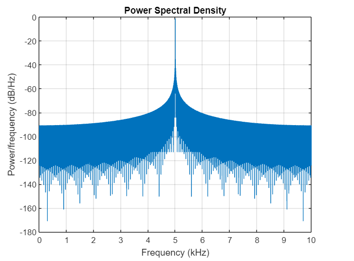
Power Spectral Density Curve

Derivation of Power Spectral Density (PSD)

Consider a continuous time power signal [Tex]y(t)[/Tex] which is defined as follows. Here, [Tex]x(t)[/Tex] is a power signal that is defined up to infinity.

[Tex]\therefore y(t) = x(t), \ |t| < |\frac{\tau}{2}| [/Tex]

[Tex]\therefore y(t) = 0, \ elsewhere[/Tex]

As the signal is defined for a finite duration so, the energy of the signal could be defined as follows:

[Tex]\therefore E = \int_{-\infty}^{\infty} |y(t)|^2 dt[/Tex]

Now, defining the energy expression in Fourier Domain.

[Tex]\therefore E = \frac{1}{2\pi} \int_{-\infty}^{\infty} |Y(\omega)|^2 d\omega[/Tex]

As the signal [Tex]y(t) [/Tex]is defined for a range of [Tex]-\frac{\tau}{2}[/Tex] to [Tex]\frac{\tau}{2}[/Tex] So,

[Tex]\therefore \int_{-\infty}^{\infty} |y(t)|^2 dt = \int_{-\frac{\tau}{2}}^{\frac{\tau}{2}} |x(t)|^2 dt[/Tex]

Now, defining its equivalent Fourier domain representation.

[Tex]\therefore \int_{-\frac{\tau}{2}}^{\frac{\tau}{2}} |x(t)|^2 dt = \frac{1}{2\pi} \int_{-\infty}^{\infty} |Y(\omega)|^2 d\omega[/Tex]

As, Total Power [Tex](P_t)[/Tex] is defined as the total energy transferred per unit time interval [Tex](\tau)[/Tex]. Mathematically, it is defined as follows:

[Tex]\therefore P_t = \frac {E}{\tau}[/Tex]

[Tex]\therefore P_t = \frac{1}{2\pi} \int_{-\infty}^{\infty} \frac{|Y(\omega)|^2}{\tau} d\omega[/Tex]

Now, when [Tex]\tau \rightarrow \infty[/Tex] then the Total Power [Tex](P_t)[/Tex] is termed as Average Power [Tex](P_{avg})[/Tex] which is defined with the following expression:

[Tex]\therefore P_{avg} = \frac{1}{2\pi} \int_{-\infty}^{\infty} lim_{\tau \to \infty} \frac{|Y(\omega)|^2}{\tau} d\omega[/Tex]

when [Tex]\tau \to \infty[/Tex] then the expression [Tex](\frac{|Y(\omega)|}{\tau} )[/Tex] tends to a finite value. Considering that finite term to be [Tex]S(\omega)[/Tex]

[Tex]\therefore S(\omega) = lim_{\tau \to \infty} \frac{|Y(\omega)|}{\tau}[/Tex]

Hence, the expression defined above is termed as Power Spectral Density (PSD) of the continuous time signal [Tex]y(t)[/Tex]. Also, defining in terms of [Tex]X(\omega)[/Tex]

[Tex]\therefore S(\omega) = lim_{\tau \to \infty} \frac{|X(\omega)|}{\tau}[/Tex]

So, the Average Power [Tex](P_{avg})[/Tex] of the generalized continuous time signal [Tex]x(t)[/Tex] in terms of Power Spectral Density [Tex](S(\omega))[/Tex] is expressed as follows

[Tex]\therefore P_{avg} = \frac{1}{2\pi}\int_{-\infty}^{\infty} S_x(\omega) d\omega = \int_{-\infty}^{\infty} S_x(f) df[/Tex]

Characteristics of Power Spectral Density (PSD)

• It describes the power distribution or the strength of the signal over a range of frequencies.
• The shape of the plot gives an important characteristics like narrower peak describes that most of the power of the signal is concentrated at this particular frequency whereas broader peak describes that most of the power of the signal is distributed over a wide range of frequencies.
• The peak value in the plot represents the frequencies having higher or greater power level.
• It also helps in determining the bandwidth of the signal which refers to the range of the frequencies over which the energy is distributed. The plot having wider bandwidth denotes that the signal energy is distributed over wide range of frequencies.

Properties of Power Spectral Density (PSD)

Properties of Power Spectral Density given below :

1. Symmetric Property
2. Relation Between PSD and Autocorrelation Function
3. Relation Between Input and Output PSD of LTI System
4. Relation Between Power and Power Spectral Density (PSD)

Property 1: Symmetric Property

For the real valued signal the Power Spectral Density (PSD) [Tex]S(\omega)[/Tex] is symmetric i.e. even function and mathematically expressed as: [Tex]S(\omega) = S(-\omega)[/Tex].

Property 2: Relation Between PSD and Autocorrelation Function

For wide sense stationary process the Power Spectral Density (PSD) [Tex]S(\omega)[/Tex] and Autocorrelation [Tex]R(\tau)[/Tex] of a signal represents Fourier Transform pair and mathematically it can be expressed with the following expression as follows for the continuous time signal [Tex]x(t)[/Tex]:

[Tex]\therefore R_x(\tau) \longleftrightarrow \mathcal{F}[S_x(\omega)][/Tex]

[Tex]\therefore R_x(\tau) = \frac{1}{2\pi}\int_{-\infty}^{\infty} S_x(\omega) e^{i\omega \tau} d\omega = \int_{-\infty}^{\infty} S_x(f) e^{2\pi if\tau} df [/Tex]

Similarly, for a discrete time signal [Tex]x[n][/Tex] the relation between Power Spectral Density [Tex]S_x(\omega)[/Tex] and autocorrelation function [Tex]R_x[m][/Tex] can be given as:

[Tex]\therefore S_x(e^{i\omega}) = \sum_{m=-\infty}^{\infty} R_x[m]e^{-i\omega m}[/Tex]

Property 3: Relation Between Input and Output PSD of LTI System

If [Tex]x(t)[/Tex] is a signal which is given an input for Linear Time Invariant (LTI) system with an impulse response [Tex]h(t)[/Tex] then the input and the output Power Spectral Density (PSD) [Tex]S(\omega)[/Tex] can be related as follows:

[Tex]\therefore S_y(\omega) = |H(\omega)|^2 * S_x(\omega)[/Tex]

Property 4: Relation Between Power and Power Spectral Density (PSD)

The relation between Power Spectral Density (PSD) [Tex]S(\omega)[/Tex] and the power of the continuous signal [Tex]x(t)[/Tex] can be expressed as follows:

[Tex]\therefore P_x = \frac{1}{2\pi}\int_{-\infty}^{\infty} S_x(\omega) d\omega = \int_{-\infty}^{\infty} S_x(f) df[/Tex]

Now, in case of discrete signal [Tex]x[n][/Tex] the expression is described as below. The expression is similar to that of the continuous one but, here the integral is performed over a range of [Tex]\omega[/Tex] from [Tex]-\pi[/Tex] to [Tex]\pi[/Tex] instead of [Tex]-\infty[/Tex] to [Tex]\infty[/Tex]. Also, here [Tex]\omega[/Tex] is normalized by sampling frequency [Tex](f_s)[/Tex] such that [Tex]\omega = 2\pi \frac{f}{f_s}[/Tex].

[Tex]\therefore P_x = \frac{1}{2\pi}\int_{-\pi}^{\pi} S_x(e^{i\omega}) d\omega = \int_{-\frac{fs}{2}}^{\frac{fs}{2}} S_x(f) df[/Tex]

Solved Problems

Consider a signal [Tex]x(t)[/Tex] whose power spectral density can be given as [Tex]S_x(f) = \frac{1}{4\pi} e^{-2\pi |f|}[/Tex]. Then (a) Find the Autocorrelation function [Tex]R_x(\tau)[/Tex] of signal [Tex]x(t)[/Tex]. (b) Determine the total power of the signal [Tex]x(t)[/Tex].

a) As known that the power spectral density and the autocorrelation function represents Fourier transform pairs. So,

[Tex]\therefore R_x(\tau) = \int_{-\infty}^{\infty} S_x(f) e^{2\pi if\tau} df [/Tex]

[Tex]\therefore R_x(\tau) = \int_{-\infty}^{\infty} \frac{1}{4\pi} e^{-2\pi |f|} e^{2\pi if\tau} df[/Tex]

[Tex]\therefore R_x(\tau) = \frac{1}{4\pi} \int_{-\infty}^{\infty} e^{-2\pi |f|} e^{2\pi if\tau} df[/Tex]

[Tex]\therefore R_x(\tau) = \frac{1}{4\pi} \int_{-\infty}^{0} e^{-2\pi (-f)} e^{2\pi if\tau} df + \frac{1}{4\pi} \int_{0}^{\infty} e^{-2\pi (+f)} e^{2\pi if\tau} df [/Tex]

[Tex]\therefore R_x(\tau) = \frac{1}{4\pi} \int_{-\infty}^{0} e^{2\pi (i\tau f + f)} df + \frac{1}{4\pi} \int_{0}^{\infty} e^{2\pi (i\tau f-f)} df [/Tex]

[Tex]\therefore R_x(\tau) = \frac{1}{4\pi} [ \frac{e^{2\pi (i\tau f + f)}}{2\pi (i\tau +1)} |_{-\infty}^{0}] + \frac{1}{4\pi} [ \frac{e^{2\pi (i\tau f – f)}}{2\pi (i\tau – 1)} |_{0}^{\infty}] [/Tex]

Now, as [Tex]1 >> i\tau[/Tex] so the limit converges to 0 near [Tex]+\infty[/Tex] and also [Tex]lim_{x\to\infty} e^{-x} = 0[/Tex].

[Tex]\therefore R_x(\tau) = \frac{1}{4\pi} [ \frac{1}{2\pi (i\tau +1)}] + \frac{1}{4\pi} [ \frac{-1}{2\pi (i\tau – 1)}] [/Tex]

[Tex]\therefore R_x(\tau) = \frac{1}{8\pi^{2}} [ \frac{1}{ (1+i\tau)} + \frac{1}{ (1-i\tau )}] [/Tex]

[Tex]\therefore R_x(\tau) = \frac{1}{8\pi^{2}} [ \frac{2}{ (1^{2}-(i\tau)^{2})}] [/Tex]

As, [Tex]i^{2} = -1[/Tex]

[Tex]\therefore R_x(\tau) = \frac{1}{8\pi^{2}} [ \frac{2}{ (1-((-1)(\tau)^{2})}] [/Tex]

[Tex]\therefore R_x(\tau) = \frac{1}{4\pi^{2}} [ \frac{1}{ 1+\tau^{2}}] [/Tex]

b) Now, the total power of the signal is given as follows

[Tex]\therefore P_x = \frac{1}{2\pi}\int_{-\infty}^{\infty} S_x(\omega) d\omega = \int_{-\infty}^{\infty} S_x(f) df[/Tex]

[Tex]\therefore P_x = \int_{-\infty}^{\infty} \frac{1}{4\pi} e^{-2\pi |f|} df[/Tex]

[Tex]\therefore P_x = \frac{1}{4\pi} \int_{-\infty}^{\infty} e^{-2\pi |f|} df[/Tex]

As [Tex]e^{-2\pi |f|}[/Tex] is an even function i.e. symmetric about y-axis. So, using the property of even function

[Tex]\therefore \int_{-\infty}^{\infty} e^{-2\pi |f|} df = 2\int_{0}^{\infty}e^{-2\pi f} df[/Tex]

[Tex]\therefore P_x = \frac{1}{4\pi} .2\int_{0}^{\infty} e^{-2\pi f} df[/Tex]

[Tex]\therefore P_x = \frac{1}{2\pi} \int_{0}^{\infty} e^{-2\pi f} df[/Tex]

[Tex]\therefore P_x = \frac{1}{2\pi} [\frac{e^{-2\pi f}}{-2\pi}|_{0}^{\infty}][/Tex]

As, [Tex]lim_{x\to\infty} e^{-x} = 0[/Tex]

[Tex]\therefore P_x = \frac{1}{2\pi} [\frac{-1}{-2\pi}][/Tex]

[Tex]\therefore P_x = \frac{1}{4\pi^{2}}[/Tex] Watt

Applications of Power Spectral Density

• Signal Processing: PSD concept is used to extract relevant information from the signals for pattern recognition and various machine learning techniques. PSD is also used in the field of telecommunication for signal classification. it is also used for noise analysis as well from the PSD distribution.
• Communications: In the field of communication PSD is used for optimizing spectral efficiency and it also helps to characterize frequency selective fading of communication channels.
• Audio Processing: It is used for noise reduction and for equalizing in the field of audio processing.
• Biomedical Signal Processing: PSD analysis of the Electroencephalography (EEG) helps one to study about the brain activity and PSD can also be used for measuring heart rate variability.
• Environmental Monitoring: PSD analysis of environmental sounds could help one understand about different wildlife habitats and for identifying different species.

Conclusion

In short, Power Spectral Density is a distribution which tells about the average power distribution over a range of frequency components. Due to its importance it has lots of application in various fields such as signal processing, communications, audio processing, biomedical signal processing and many such related fields. A popular property of PSD also stated as Wiener Khinchin Theorem states that autocorrelation and PSD distribution of a signal are Fourier Transform pairs of each other.

FAQs on Power Spectral Density

What are the limitations or assumptions of Power Spectral Density?

The main underlying assumptions or limitations of PSD is that it assumes a signal to be stationary i.e. a signal whose properties does not change with time. For the analysis of the non-stationary signals the time varying techniques like spectrogram is generally preferred for analysis.

How PSD is used for noise analysis?

One need to take special care while interpreting the results of PSD in noisy environments. In noisy environment PSD distribution tells about the frequencies contributing to noise component. This analysis is very useful in filtering techniques and while designing effective noise suppression.

Can PSD help in determining stability of the system?

Yes, PSD analysis can be used for determining the stability of the system especially in the control system as well as feedback systems by analyzing its frequency response.

Is PSD applicable to both continuous as well as discrete time signals?

Yes, PSD can be applied to both continuous as well as discrete time signals. For discrete time signals PSD is estimated using periodogram or Welch method after doing sampling process.

What are the software or tools for PSD analysis?

There are many such software and tools for PSD analysis, and popular one among them are namely MATLAB, Python’s SciPy and many other specialized signal processing packages or libraries for its analysis.