Model with Reduction Methods

Machine learning models are now more powerful and sophisticated than ever before, able to handle challenging problems and enormous datasets. But with great power also comes huge complexity, and occasionally these models grow too complicated to be useful for implementation in the real world. Methods of model reduction are useful in this situation. This article will discuss the idea of model reduction in machine learning, explaining it simply for newcomers, clarifying essential terms, and providing concrete Python examples to show how it works. We will introduce some common dimensionality reduction techniques and show how to apply them to a machine-learning model using Python.

What is Model Reduction?

In the context of machine learning, the practice of reducing complicated models while maintaining their critical predictive skills is referred to as model reduction. It’s comparable to condensing a complex map into one that is still usable for navigation. By balancing model simplicity with prediction accuracy, these reduction techniques attempt to improve the model’s interpretability, computational efficiency, and suitability for deployment in situations with limited resources.

Primary Terminologies

Before diving deeper, let’s define some key terms:

1. Machine Learning Model: A computational model that learns patterns from data to make predictions or decisions.
2. Model Complexity: The intricacy of a machine learning model, often measured by the number of parameters and features.
3. Model Reduction: The process of simplifying a complex machine learning model while preserving its predictive performance.
4. Overfitting: When a model is too complex and fits the training data too closely, leading to poor generalization to new, unseen data.
5. Interpretability: The ease with which humans can understand and explain how a model makes predictions.
6. Computational Efficiency: The ability of a model to make predictions quickly and with minimal computational resources.

Concepts Related to Model Reduction

1. Occam’s Razor: Occam’s Razor, a principle often applied in model reduction, suggests that among competing hypotheses, the simpler one is usually the correct one. In machine learning, this translates to preferring simpler models when they perform as well as, or almost as well as, complex ones.
2. Feature Selection: One way to reduce model complexity is by selecting a subset of the most informative features (input variables) for training. This reduces the dimensionality of the data and can improve model performance.
3. Dimensionality Reduction: Dimensionality reduction techniques like Principal Component Analysis (PCA) and t-Distributed Stochastic Neighbor Embedding (t-SNE) aim to project high-dimensional data into a lower-dimensional space while preserving essential information. This simplifies the model without significant loss of information.

Dimensionality Reduction Techniques

Feature selection and feature extraction are the two primary categories of dimensionality reduction approaches. A subset of the original characteristics that are most pertinent or significant to the current issue are chosen through feature selection. Feature extraction entails merging or otherwise altering the source features to produce new features. Some of the popular feature selection methods are:

Filter techniques: These approaches, such as correlation, variance, or information gain, rank the characteristics according to how relevant they are to the target variable. The highest-scoring elements are chosen, while the remainder are disregarded.

Wrapper methods: The “wrapper” approach chooses features based on how well the model performs. They experiment with various feature combinations and assess how well they match the model. The attributes that provide the best model are chosen, and the others are disregarded.

Embedded methods: Techniques that incorporate feature selection and model training are referred to as embedded techniques. To choose the characteristics that are most advantageous for the model, they employ regularization methods like decision trees.

Model Reduction Methods with example

1. Feature Selection

Concept: Feature selection involves choosing the most relevant features (input variables) for a model while discarding less important ones. Various techniques, like statistical tests (ANOVA F-statistic), rank features based on their relevance to the target variable. Feature selection is the process of choosing the most relevant features (input variables) for training a model while discarding less important ones. This reduces the dimensionality of the data and can improve model performance.

Python Example:

Python

import matplotlib.pyplot as plt
import numpy as np
from sklearn.datasets import load_iris
from sklearn.tree import DecisionTreeClassifier
from sklearn.model_selection import train_test_split
from sklearn.metrics import accuracy_score
from sklearn.feature_selection import SelectKBest, f_classif

# Load the Iris dataset
data = load_iris()
X, y = data.data, data.target

# Split data into training and testing sets
X_train, X_test, y_train, y_test = train_test_split(X, y, test_size=0.2, random_state=42)

# Function to plot decision boundaries
def plot_decision_boundary(model, X, y):
    h = 0.02  # Step size in the mesh
    x_min, x_max = X[:, 0].min() - 1, X[:, 0].max() + 1
    y_min, y_max = X[:, 1].min() - 1, X[:, 1].max() + 1
    xx, yy = np.meshgrid(np.arange(x_min, x_max, h), np.arange(y_min, y_max, h))

    Z = model.predict(np.c_[xx.ravel(), yy.ravel()])
    Z = Z.reshape(xx.shape)

    plt.contourf(xx, yy, Z, cmap=plt.cm.RdYlBu, alpha=0.6)
    plt.scatter(X[:, 0], X[:, 1], c=y, cmap=plt.cm.RdYlBu)
    plt.xlabel("Feature 1")
    plt.ylabel("Feature 2")
    plt.title("Decision Boundary")

# Create a complex decision tree model
complex_model = DecisionTreeClassifier()
complex_model.fit(X_train[:, :2], y_train)  # We'll use only the first two features for visualization

# Feature selection: Select the top two most relevant features
selector = SelectKBest(score_func=f_classif, k=2)
X_train_reduced = selector.fit_transform(X_train, y_train)
X_test_reduced = selector.transform(X_test)

# Create a decision tree model using reduced features
model_with_reduced_features = DecisionTreeClassifier()
model_with_reduced_features.fit(X_train_reduced, y_train)

# Plot decision boundaries
plt.figure(figsize=(15, 4))
plt.subplot(1, 3, 1)
plot_decision_boundary(complex_model, X_train[:, :2], y_train)
plt.title("Complex Decision Tree (All Features)")

plt.subplot(1, 3, 2)
plot_decision_boundary(model_with_reduced_features, X_train_reduced, y_train)
plt.title("Decision Tree with Reduced Features")

# Calculate accuracy for both models
y_pred_complex = complex_model.predict(X_test[:, :2])
accuracy_complex = accuracy_score(y_test, y_pred_complex)
y_pred_reduced = model_with_reduced_features.predict(X_test_reduced)
accuracy_reduced = accuracy_score(y_test, y_pred_reduced)

plt.subplot(1, 3, 3)
plt.bar(['Complex Model', 'Reduced Model'], [accuracy_complex, accuracy_reduced], color=['blue', 'orange'])
plt.ylim(0, 1)
plt.ylabel('Accuracy')
plt.title('Model Accuracy')

plt.tight_layout()
plt.show()

Output:

You’ll see two side-by-side graphs that compare the sophisticated and simplified models’ decision bounds. The simpler model will have smoother, easier to understand choice boundaries than the complicated model, which is likely to have convoluted limits.

This graphic demonstrates how model reduction lowers the decision limits, possibly improving the model’s suitability for practical application and making it easier to understand.

Bonus Example :

Python

from sklearn.datasets import load_iris
from sklearn.feature_selection import SelectKBest, f_classif
import matplotlib.pyplot as plt

# Load the Iris dataset
data = load_iris()
X, y = data.data, data.target

# Perform feature selection using ANOVA F-statistic
num_features = X.shape[1]
selected_features = []

# Create an animation to show feature selection
for k in range(1, min(3, num_features) + 1):  # Ensure k is at most 2 for visualization
    selector = SelectKBest(score_func=f_classif, k=k)
    X_new = selector.fit_transform(X, y)
    selected_features.append(selector.get_support())
    plt.figure(figsize=(12, 4))
    plt.subplot(1, 2, 1)
    plt.scatter(X[:, 0], X[:, 1], c=y, cmap=plt.cm.coolwarm)
    plt.xlabel('Feature 0')
    plt.ylabel('Feature 1')
    plt.title(f'Original Data ')

    plt.subplot(1, 2, 2)
    if X_new.shape[1] > 1:
        plt.scatter(X_new[:, 0], X_new[:, 1], c=y, cmap=plt.cm.coolwarm)
    plt.xlabel(f'Selected Features (k={k})')
    plt.ylabel(f'Selected Features (k={k})')
    plt.title(f'Selected Features (k={k})')

    plt.tight_layout()
    plt.show()

Output:

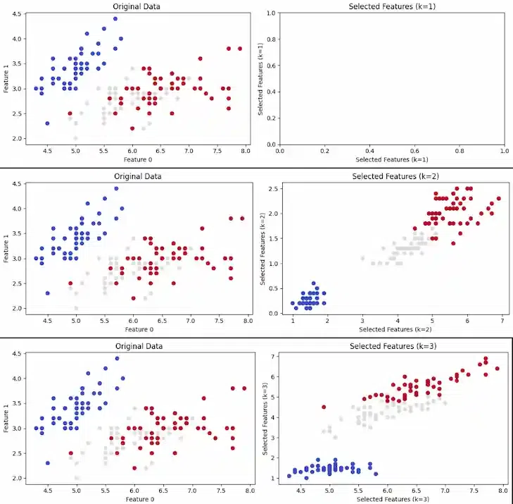
SelectKBest -Geeksforgeeks

2. Dimensionality Reduction (PCA):

Concept: Principal Component Analysis (PCA), for example, aims to project high-dimensional data into a lower-dimensional space while maintaining critical information. This streamlines the model without seriously compromising its accuracy. By identifying a set of orthogonal axes (principal components) along which the data fluctuates most, Principal Component Analysis (PCA) decreases the dimensionality of the data. This technique reduces the number of dimensions while keeping crucial information by projecting data onto these components.

Python Example:

Python

from sklearn.decomposition import PCA

# Apply PCA for dimensionality reduction (reduce to 2 components)
pca = PCA(n_components=2)
X_train_pca = pca.fit_transform(X_train)
X_test_pca = pca.transform(X_test)

# Create a decision tree model using PCA-reduced data
model_with_pca = DecisionTreeClassifier()
model_with_pca.fit(X_train_pca, y_train)

# Plot decision boundaries
plt.figure(figsize=(15, 4))
plt.subplot(1, 3, 1)
plot_decision_boundary(complex_model, X_train[:, :2], y_train)
plt.title("Complex Decision Tree (All Features)")

plt.subplot(1, 3, 2)
plot_decision_boundary(model_with_pca, X_train_pca, y_train)
plt.title("Decision Tree with PCA-Reduced Features")

# Calculate accuracy for both models
y_pred_pca = model_with_pca.predict(X_test_pca)
accuracy_pca = accuracy_score(y_test, y_pred_pca)

plt.subplot(1, 3, 3)
plt.bar(['Complex Model', 'PCA-Reduced Model'], [accuracy_complex, accuracy_pca], color=['blue', 'green'])
plt.ylim(0, 1)
plt.ylabel('Accuracy')
plt.title('Model Accuracy')

plt.tight_layout()
plt.show()

Output:

In this code, we apply PCA to reduce the dimensionality of the data to just two principal components. We then train a decision tree model using these reduced components and visualize the decision boundary.

By comparing the decision boundaries in both cases (feature selection and PCA), you can see how these model reduction methods simplify the model while retaining the essential patterns in the data.

Bonus Example:

Python

from sklearn.decomposition import PCA
from sklearn.datasets import load_iris
import matplotlib.pyplot as plt

# Load the Iris dataset
data = load_iris()
X, y = data.data, data.target

# Perform PCA for dimensionality reduction
pca = PCA(n_components=2)
X_pca = pca.fit_transform(X)

# Create an animation to show PCA in action
plt.figure(figsize=(12, 4))
plt.subplot(1, 2, 1)
plt.scatter(X[:, 0], X[:, 1], c=y, cmap=plt.cm.coolwarm)
plt.xlabel('Feature 0')
plt.ylabel('Feature 1')
plt.title(f'Original Data')

plt.subplot(1, 2, 2)
plt.scatter(X_pca[:, 0], X_pca[:, 1], c=y, cmap=plt.cm.coolwarm)
plt.xlabel('Principal Component 1')
plt.ylabel('Principal Component 2')
plt.title(f'PCA Reduced Data (k=2)')

plt.tight_layout()
plt.show()

Output:

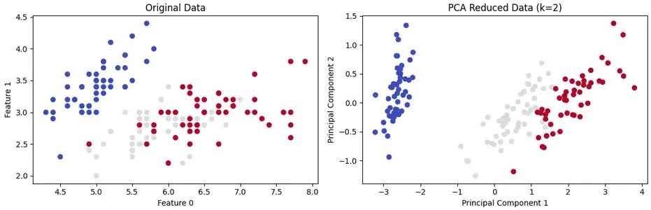
Feature Reduction using PCA

3. Regularization

Concept: Regularization involves adding constraints to a model to prevent it from becoming too complex. One common approach is to limit the maximum depth of a decision tree, effectively simplifying the tree’s structure.

Python Example:

Python

import numpy as np
import matplotlib.pyplot as plt
from sklearn.datasets import make_moons
from sklearn.tree import DecisionTreeClassifier
from sklearn.model_selection import train_test_split
from sklearn.metrics import accuracy_score

# Generate the dataset
X, y = make_moons(n_samples=300, noise=0.25, random_state=42)

# Split data into training and testing sets
X_train, X_test, y_train, y_test = train_test_split(X, y, test_size=0.3, random_state=42)

# Create a complex decision tree model
complex_model = DecisionTreeClassifier(random_state=42)
complex_model.fit(X_train, y_train)

# Create a regularized decision tree model with limited depth
regularized_model = DecisionTreeClassifier(max_depth=3, random_state=42)
regularized_model.fit(X_train, y_train)

# Calculate accuracy for both models
y_pred_complex = complex_model.predict(X_test)
accuracy_complex = accuracy_score(y_test, y_pred_complex)

y_pred_regularized = regularized_model.predict(X_test)
accuracy_regularized = accuracy_score(y_test, y_pred_regularized)

# Plot decision boundaries
def plot_decision_boundary(model, X, y, ax, title):
    h = 0.02
    x_min, x_max = X[:, 0].min() - 1, X[:, 0].max() + 1
    y_min, y_max = X[:, 1].min() - 1, X[:, 1].max() + 1
    xx, yy = np.meshgrid(np.arange(x_min, x_max, h), np.arange(y_min, y_max, h))
    Z = model.predict(np.c_[xx.ravel(), yy.ravel()])
    Z = Z.reshape(xx.shape)
    ax.contourf(xx, yy, Z, cmap=plt.cm.RdYlBu, alpha=0.6)
    ax.scatter(X[:, 0], X[:, 1], c=y, cmap=plt.cm.RdYlBu)
    ax.set_xlabel("Feature 1")
    ax.set_ylabel("Feature 2")
    ax.set_title(title)

plt.figure(figsize=(12, 4))
plt.subplot(1, 3, 1)
plot_decision_boundary(complex_model, X, y, plt.gca(), "Complex Decision Tree (No Regularization)")

plt.subplot(1, 3, 2)
plot_decision_boundary(regularized_model, X, y, plt.gca(), "Regularized Decision Tree (Max Depth = 3)")

# Display accuracy comparison
plt.subplot(1, 3, 3)
plt.bar(['Complex Model', 'Regularized Model'], [accuracy_complex, accuracy_regularized], color=['blue', 'purple'])
plt.ylim(0, 1)
plt.ylabel('Accuracy')
plt.title('Model Accuracy Comparison')
plt.tight_layout()
plt.show()

Output:

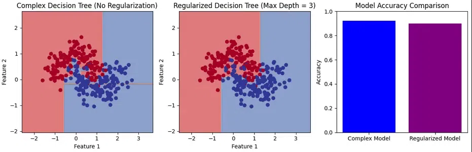
Model Reduction

In this example, we use the make_moons dataset, which is nonlinear and not linearly separable. You will notice that the complex model (without regularization) overfits the data, while the regularized model (with limited depth) has a more generalized decision boundary. This clearly demonstrates the effect of regularization in simplifying the model and improving its ability to generalize to unseen data.

Regularization (L1 and L2)

Regularization is a method to reduce model complexity by adding penalties to the model’s loss function based on the magnitude of its parameters (weights). L1 regularization (Lasso) adds a penalty proportional to the absolute values of the parameters, which can lead some parameters to become exactly zero. L2 regularization (Ridge) adds a penalty proportional to the square of parameter values, discouraging large parameter values.

Python Implementation

Python

import numpy as np
import matplotlib.pyplot as plt
from sklearn.linear_model import LogisticRegression
from sklearn import datasets
from sklearn.preprocessing import StandardScaler
from sklearn.model_selection import train_test_split

# Load the Iris dataset
iris = datasets.load_iris()
X = iris.data[:, :2]  # We'll use the first two features for simplicity
y = iris.target

# Standardize the features
scaler = StandardScaler()
X = scaler.fit_transform(X)

# Regularization paths
alphas = np.logspace(-2, 2, 50)
coefs_lasso = []
coefs_ridge = []

for alpha in alphas:
    lasso = LogisticRegression(penalty='l1', C=1/alpha, solver='liblinear', multi_class='ovr')
    ridge = LogisticRegression(penalty='l2', C=1/alpha, solver='lbfgs', multi_class='ovr')
    lasso.fit(X, y)
    ridge.fit(X, y)
    coefs_lasso.append(lasso.coef_.ravel())
    coefs_ridge.append(ridge.coef_.ravel())

# Create subplots for L1 and L2 regularization paths
plt.figure(figsize=(12, 6))
plt.subplot(121)
plt.plot(alphas, coefs_lasso)
plt.title('L1 Regularization Path (Lasso)')
plt.xlabel('Alpha (Regularization Strength)')
plt.ylabel('Coefficient Values')
plt.legend(iris.feature_names[:2])

plt.subplot(122)
plt.plot(alphas, coefs_ridge)
plt.title('L2 Regularization Path (Ridge)')
plt.xlabel('Alpha (Regularization Strength)')
plt.ylabel('Coefficient Values')
plt.legend(iris.feature_names[:2])

plt.tight_layout()
plt.show()

Output:

4. t-Distributed Stochastic Neighbor Embedding (t-SNE)

Concept: t-Distributed Stochastic Neighbor Embedding (t-SNE) is a dimensionality reduction technique that is widely used for visualizing high-dimensional data in a lower-dimensional space, typically 2D or 3D. Unlike linear techniques like Principal Component Analysis (PCA), t-SNE focuses on preserving the pairwise similarities between data points, making it particularly effective for visualizing complex, nonlinear structures in the data.

Python example :

Python

from sklearn.manifold import TSNE
from sklearn.datasets import load_iris
import matplotlib.pyplot as plt

# Load the Iris dataset
data = load_iris()
X, y = data.data, data.target

# Perform t-SNE for dimensionality reduction
tsne = TSNE(n_components=2)
X_tsne = tsne.fit_transform(X)

# Create an animation to demonstrate t-SNE
plt.figure(figsize=(5, 4))
plt.scatter(X_tsne[:, 0], X_tsne[:, 1], c=y, cmap=plt.cm.coolwarm)
plt.xlabel('t-SNE Dimension 1')
plt.ylabel('t-SNE Dimension 2')
plt.title('t-SNE for Dimensionality Reduction')
plt.show()

Output:

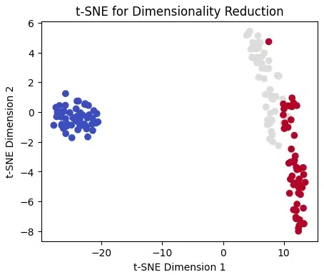
t-SNE for Dimensionality Reduction

Benefits of Model Reduction

Model reduction techniques serve several essential purposes:

• Improved Interpretability: Simplifying complex models makes them easier to understand and explain, crucial for stakeholders.
• Computational Efficiency: Reduced complexity leads to faster model training and prediction, critical in real-time applications.
• Generalization: Simpler models are less prone to overfitting and often generalize better to unseen data.

Conclusion

Model reduction is a vital technique in machine learning, allowing us to simplify complex models without sacrificing predictive performance. By applying feature selection, dimensionality reduction, or regularization, we can make our models more interpretable, computationally efficient, and better suited for real-world deployment. Understanding when and how to use these model reduction methods is essential for machine learning practitioners. This article has shown us how to use Python to apply several popular dimensionality reduction strategies to a machine learning model. We have shown that dimensionality reduction may aid in the model’s simplification, efficiency, and understandability. On a test dataset, we also evaluated how well various strategies performed and looked at how that affected the model’s accuracy. We hope that this essay has enlightened you on the subject and encouraged you to learn more. Happy studying!