Isomap for Dimensionality Reduction in Python

In the realm of machine learning and data analysis, grappling with high-dimensional datasets has become a ubiquitous challenge. As datasets grow in complexity, traditional methods often fall short of capturing the intrinsic structure, leading to diminished performance and interpretability. In this landscape, Isomap (Isometric Mapping) emerges as a potent technique designed explicitly to navigate the intricacies of complex, non-linear structures inherent in data. Dimensionality reduction is a crucial aspect of machine learning and data analysis, especially when dealing with high-dimensional datasets. One powerful technique for this purpose is Isomap, an algorithm designed to capture the underlying geometry of complex, non-linear structures. Isomap stands for Isometric Mapping, and its primary goal is to unfold intricate patterns in high-dimensional data into a lower-dimensional space while preserving the essential relationships between data points.

What is Isometric Feature Mapping (ISOMAP)?

Isomap, an abbreviation for Isometric Mapping, is a dimensionality reduction algorithm that transcends the limitations of linear approaches. Its primary objective is to unfold intricate patterns within high-dimensional data into a lower-dimensional space while meticulously preserving the essential relationships between data points. Unlike linear methods such as Principal Component Analysis (PCA), which assume a linear relationship between variables, Isomap excels at capturing the underlying non-linear structure, making it a go-to choice for a diverse array of applications.

Workings of ISOMAP?

Step 1: Construct the Neighbourhood Graph

At the core of Isomap lies a series of steps that collectively contribute to its unique ability to reveal the intrinsic geometry of complex datasets. The algorithm initiates by constructing a neighborhood graph, where nodes represent data points, and edges connect nodes that are within a certain distance of each other. A neighborhood graph is a graph where nodes are data points and edges connect nodes that are within a certain distance of each other. This neighborhood graph serves as the foundational structure for Isomap’s subsequent computations. To construct the neighborhood graph, we first calculate the Euclidean distance between all pairs of data points. Then, we select the k nearest neighbors for each data point and create edges in the graph connecting these neighbours. The value of k is a parameter of the algorithm that can be adjusted depending on the data.

Euclidean distance between all pairs of data points:

where:

• is the Euclidean distance between data points and
• is the Euclidean norm of the vector

Neighborhood graph: A graph G can be defined over the data points by connecting points i and j if they are closer than a specifiеd threshold e (e-Isomap), or if i is one of the K-nearest neighbors of j (K-Isomap).The choice of k affects the connectivity and shape of the neighborhood graph. If k is chosen too small, the neighborhood graph may not be connected, while if it is chosen too large, it may lead to a so-called “short-circuit error.”

Step 2: Approximate Geodesic Distances

Isomap then delves into the realm of geodesic distances, a concept critical to understanding the true structure of non-linear manifolds. The geodesic distance between two points in a neighborhood graph is defined as the shortest path along the edges of the graph, measuring the distance on the curved surface of a manifold. Unlike the Euclidean distance, which represents a straight-line measurement, the geodesic distance is sensitive to the underlying structure, capturing the true intricacies of the data. To approximate the geodesic distance by calculating the shortest path between the two points along the edges of the neighborhood graph variety of algorithms can be used, such as Dijkstra’s algorithm or Floyd-Warshall’s algorithm. The algorithm efficiently computes the shortest paths between all pairs of vertices in a graph.

Floyd-Warshall algorithm for finding the shortest paths in a weighted graph.

Initialize with a array Dg of minimum distances to infinity, and setting the distance from each vertex to itself as 0. For each edge (i, j), the distance in Dg should be as the weight of the edge (i, j). Finally, Iterate through all pairs of vertices (i, j) and update the distance if a shorter path is found by going through vertex k.

Step 3: Apply Multidimensional Scaling (MDS)

The final step in Isomap is to apply multidimensional scaling (MDS). MDS is a dimensionality reduction technique that aims to find a lower-dimensional representation of the data that preserves the pairwise distances between data points. Once the geodesic distances have been computed, Isomap embeds the data in a lower-dimensional space. This embedding is performed using a technique called spectral embedding. Spectral embedding is a dimensionality reduction technique that works by finding the principal components of the graph Laplacian. The graph Laplacian is a matrix that represents the connectivity of the neighborhood graph. The magic of Isomap unfolds with the application of spectral embedding. The graph Laplacian, a matrix representing the connectivity of the neighborhood graph, encapsulates the relationships and proximities between data points. By unveiling the principal components, Isomap successfully embeds the data into a lower-dimensional space while meticulously preserving the essential geometric relationships.

Geodesic Distance vs. Euclidean Distance: Unveiling the Variance in Measurement

	Euclidean Distance	Geodesic Distance
Definition	Euclidean distance is the straight-line distance between two points in Euclidean space. It represents the length of the shortest path between two points in a flat, Cartesian space.	Geodesic distance is the shortest path between two points on a curved surface, such as a manifold or graph. It accounts for the curvature or non-linearity of the space, providing a more accurate measure on non-flat surfaces.
Measurement Basis	Based on the straight-line distance formula derived from the Pythagorean theorem. Assumes a flat, linear space without considering any curvature or obstacles.	Based on the shortest path along the curved surface. Reflects the intrinsic structure of the space, considering any bends or twists.
Applicability	Appropriate for flat, Euclidean spaces. Well-suited for measuring distances in traditional Cartesian coordinate systems	Essential for measuring distances on curved surfaces, manifolds, or graphs. Suitable for capturing distances in spaces with non-linear structures.
Calculation Method	Computed using the familiar straight-line distance formula in Euclidean space. For two points (x1 ,y1) and (x2 ,y2) the Euclidean distance is given by square root ((x2-x1)2+(y2-y1)2)	Computed based on the shortest path along the curved surface. Often involves algorithms like Dijkstra’s algorithm on a graph or specialized methods for manifold spaces.
Sensitivity to Structure	Insensitive to the underlying structure of the space. Treats the space as flat and measures distances without considering bends or twists.	Sensitive to the intrinsic structure of the space. Captures the true distances, accounting for the non-linearities present.
Example	On a flat map, the Euclidean distance between two cities is a straight-line measurement.	On the surface of the Earth, the geodesic distance between two cities considers the curvature of the planet, providing a more accurate representation.
Representation in Isomap	Isomap, when using Euclidean distances, assumes a flat geometry.	Isomap, utilizing geodesic distances (shortest paths on the neighborhood graph), captures the non-linear structure of the data.
Impact on Dimensionality Reduction	May lead to inaccurate representations when dealing with non-linear manifold data.	Ensures a more accurate representation of the underlying structure, crucial for preserving relationships in non-linear spaces.

In summary, the key difference between geodesic and Euclidean distance lies in their approach to measuring distance. While Euclidean distance assumes a flat, straight-line measurement, geodesic distance considers the curvature and intricacies of the space, providing a more accurate representation, especially in non-linear or curved environments. In dimensionality reduction techniques like Isomap, the use of geodesic distances ensures a faithful portrayal of the intrinsic geometry of the data.

Advantages of ISOMAP?

• Handling Non-Linear Structures: Isomap is crucial when dealing with datasets that exhibit complex, non-linear structures or lie on non-linear manifolds. Linear dimensionality reduction methods like Principal Component Analysis (PCA) may struggle to capture the intricate patterns present in non-linear data. Isomap excels in preserving the intrinsic geometry of such complex structures, offering a more accurate representation.
• Preserving Local and Global Structure: Isomap is designed to preserve both local and global structure in the data. By leveraging geodesic distances and neighborhood graphs, Isomap ensures that relationships between nearby and distant data points are accurately maintained. This is essential for tasks where preserving the relative distances between data points is critical, such as manifold learning.
• Versatility Across Applications: Isomap finds applications in diverse domains, including image classification, video compression, fraud detection, and natural language processing. Its ability to uncover complex structures makes Isomap versatile for various tasks. Whether reducing dimensionality for image data, compressing videos, identifying fraud in transactions, or preprocessing text for natural language processing, Isomap adapts to different data types and structures.

Disadvantages of ISOMAP?

• Computation of pairwise geodesic distances, can be computationally expensive, especially for large datasets.
• Sensitive to noise and outliers in the data, leading to distorted embeddings.
• ISOMAP may suffer from the curse of dimensionality, particularly when the intrinsic dimensionality is not well-defined.
• ISOMAP can be influenced by the choice of the neighborhood size or the number of nearest neighbors, and finding an optimal value may be challenging.

Applications of Isomap

Isomap can be used for a variety of tasks, including:

• image classification: Use isomap to decrease the dimensionality of picture data before training a classifier. This can increase the classifier’s performance while also shortening the training time.
• Video compression: Before reducing video data, isomap can be employed to minimise its dimensionality. This can lower the size of the compressed video file while maintaining quality.
• Fraud detection: Isomap has the ability to detect fraudulent transactions. Isomap, for example, may be used to identify transactions that are far apart in the geodesic space.
• Natural language processing: Before doing natural language processing activities such as sentiment analysis or topic modelling, Isomap may be used to decrease the dimensionality of text input.

Visualizing Handwritten Digits with Isomap Dimensionality Reduction

Step 1: Importing Libraries

Python

import numpy as np
import matplotlib.pyplot as plt
from sklearn.datasets import load_digits
from sklearn.manifold import Isomap
from sklearn.preprocessing import StandardScaler
from sklearn.pipeline import Pipeline

Step 2: Dataset Loading and Preprocessing

Python

digits = load_digits()
X, y = digits.data, digits.target
scaler = StandardScaler()
X_standardized = scaler.fit_transform(X)

Step 3: Apply Isomap for Dimensionality Reduction

The code creates an Isomap model with 30 neighbors and 2 output dimensions, then fits the model to the standardized input data and transforms it into the lower-dimensional space.

Python

isomap = Isomap(n_neighbors=30, n_components=2)
X_transformed = isomap.fit_transform(X_standardized)

Step 4: Plot the reduced-dimensional data

The code creates a scatter plot of the data points visualizing the 2D representation of handwritten digits from the MNIST dataset, with each digit class represented by a different color. The plot includes a color bar for reference.

Python3

plt.figure(figsize=(10, 8))
scatter = plt.scatter(X_transformed[:, 0], X_transformed[:, 1], c=y, cmap='viridis', edgecolors='k', s=20)
plt.title('Isomap - 2D Representation of Handwritten Digits (MNIST)')
plt.xlabel('Component 1')
plt.ylabel('Component 2')
plt.colorbar(scatter, ticks=np.arange(10), label='Digit Class')

plt.show()

Output:

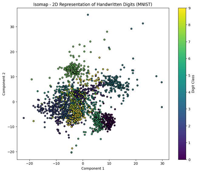Here, Each digit class is represented by a different color, revealing distinct clusters corresponding to the different digits. This visualization demonstrates the effectiveness of Isomap in preserving the underlying structure of the data while reducing its dimensionality.

Conclusion

Isomap is a versatile dimensionality reduction approach. It is especially well-suited for data on a non-linear manifold, such as photos, videos, or text.