Matplotlib.pyplot.streamplot() in Python

Stream plot is basically a type of 2D plot used majorly by physicists to show fluid flow and 2D field gradients .The basic function to create a stream plot in Matplotlib is: 

ax.streamplot(x_grid, y_grid, x_vec, y_vec, density=spacing)

Here x_grid and y_grid are arrays of the x and y points.The x_vec and y_vec represent the stream velocity of each point present on the grid.The attribute #density=spacing# specify that how much close the streamlines are to be drawn together.

Creating stream plot –

Let’s start by creating a simple stream plot that contains streamlines on a 10 by 10 grid.All the streamlines are parallel and pointing towards the right.The code below creates the stream plot containing horizontal parallel lines pointing to the right: 

Python3

# Import libraries
import numpy as np
import matplotlib.pyplot as plt

# Creating dataset
x = np.arange(0, 10)
y = np.arange(0, 10)

# Creating grids
X, Y = np.meshgrid(x, y)

# x-component to the right
u = np.ones((10, 10))

# y-component zero
v = np.zeros((10, 10))

fig = plt.figure(figsize = (12, 7))

# Plotting stream plot
plt.streamplot(X, Y, u, v, density = 0.5)

# show plot
plt.show()

Output:

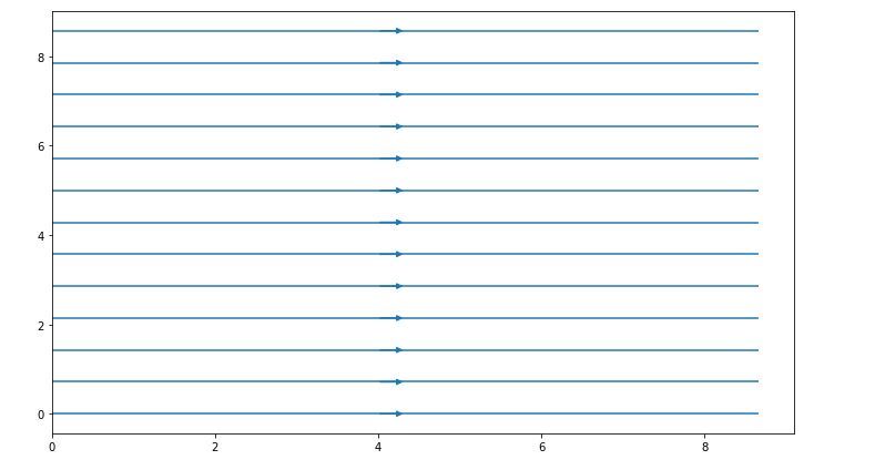
Here, x and y are 1D arrays on an evenly spaced grid, u and v are 2D arrays of velocities of x and y where the number of rows should match with the length of y while the number of columns should match with x, density is a float value which controls the closeness of the stream lines.

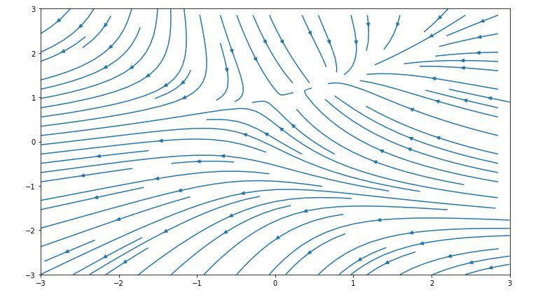
Customization of stream plot –

With the help of streamplot() function we can create and customize a plot showing field lines based on defined 2D vector field. Many attributes are available in streamplot() function for the modification of the plots.

Python3

# Import libraries
import numpy as np
import matplotlib.pyplot as plt

# Creating data set
w = 3
Y, X = np.mgrid[-w:w:100j, -w:w:100j]
U = -1 - X**2 + Y
V = 1 + X - Y**2
speed = np.sqrt(U**2 + V**2)

# Creating plot
fig = plt.figure(figsize = (12, 7))
plt.streamplot(X, Y, U, V, density = 1)

# show plot
plt.show()

Output:

Some of the customization of the above graph are listed below:
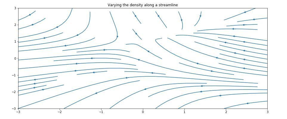
Varying the density of streamlines –

Python3

import numpy as np
import matplotlib.pyplot as plt
import matplotlib.gridspec as gridspec

# Creating dataset
w = 3
Y, X = np.mgrid[-w:w:100j, -w:w:100j]
U = -1 - X**2 + Y
V = 1 + X - Y**2
speed = np.sqrt(U**2 + V**2)

fig = plt.figure(figsize =(24, 20))
gs = gridspec.GridSpec(nrows = 3, ncols = 2,
                       height_ratios =[1, 1, 2])

# Varying the density along a
# streamline
ax = fig.add_subplot(gs[0, 0])
ax.streamplot(X, Y, U, V,
              density =[0.4, 0.8])

ax.set_title('Varying the density along a streamline')

# show plot
plt.tight_layout()
plt.show()

Output:

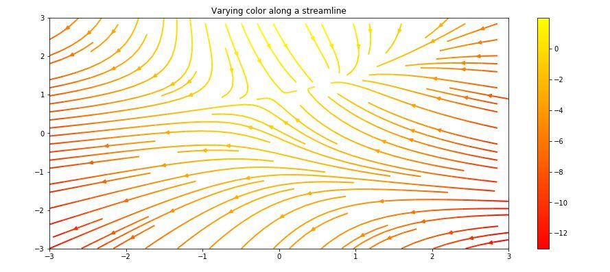
Varying the color along a streamline –

Python3

import numpy as np
import matplotlib.pyplot as plt
import matplotlib.gridspec as gridspec

# Creating dataset
w = 3
Y, X = np.mgrid[-w:w:100j, -w:w:100j]
U = -1 - X**2 + Y
V = 1 + X - Y**2
speed = np.sqrt(U**2 + V**2)

fig = plt.figure(figsize =(24, 20))
gs = gridspec.GridSpec(nrows = 3, ncols = 2,
                       height_ratios =[1, 1, 2])

# Varying color along a streamline
ax = fig.add_subplot(gs[0, 1])
strm = ax.streamplot(X, Y, U, V, color = U,
                     linewidth = 2, cmap ='autumn')
fig.colorbar(strm.lines)
ax.set_title('Varying the color along a streamline.')

# show plot
plt.tight_layout()
plt.show()

Output:

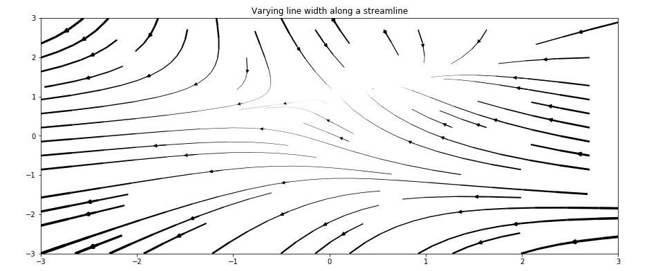
Varying the line width along a streamline –

Python3

import numpy as np
import matplotlib.pyplot as plt
import matplotlib.gridspec as gridspec

# Creating dataset
w = 3
Y, X = np.mgrid[-w:w:100j, -w:w:100j]
U = -1 - X**2 + Y
V = 1 + X - Y**2
speed = np.sqrt(U**2 + V**2)

fig = plt.figure(figsize =(24, 20))
gs = gridspec.GridSpec(nrows = 3, ncols = 2,
                       height_ratios =[1, 1, 2])

# Varying line width along a streamline
ax = fig.add_subplot(gs[1, 0])
lw = 5 * speed / speed.max()
ax.streamplot(X, Y, U, V, density = 0.6,
              color ='k', linewidth = lw)

ax.set_title('Varying line width along a streamline')

# show plot
plt.tight_layout()
plt.show()

Output:

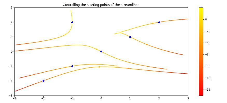
Controlling the starting points of streamlines –

Python3

import numpy as np
import matplotlib.pyplot as plt
import matplotlib.gridspec as gridspec

# Creating dataset
w = 3
Y, X = np.mgrid[-w:w:100j, -w:w:100j]
U = -1 - X**2 + Y
V = 1 + X - Y**2
speed = np.sqrt(U**2 + V**2)

fig = plt.figure(figsize =(24, 20))
gs = gridspec.GridSpec(nrows = 3, ncols = 2,
                       height_ratios =[1, 1, 2])

# Controlling the starting points
# of the streamlines
seek_points = np.array([[-2, -1, 0, 1, 2, -1],
                        [-2, -1,  0, 1, 2, 2]])

ax = fig.add_subplot(gs[1, 1])
strm = ax.streamplot(X, Y, U, V, color = U,
                     linewidth = 2,
                     cmap ='autumn',
                     start_points = seek_points.T)

fig.colorbar(strm.lines)
ax.set_title('Controlling the starting\
points of the streamlines')

# Displaying the starting points
# with blue symbols.
ax.plot(seek_points[0], seek_points[1], 'bo')
ax.set(xlim =(-w, w), ylim =(-w, w))

# show plot
plt.tight_layout()
plt.show()

Output:

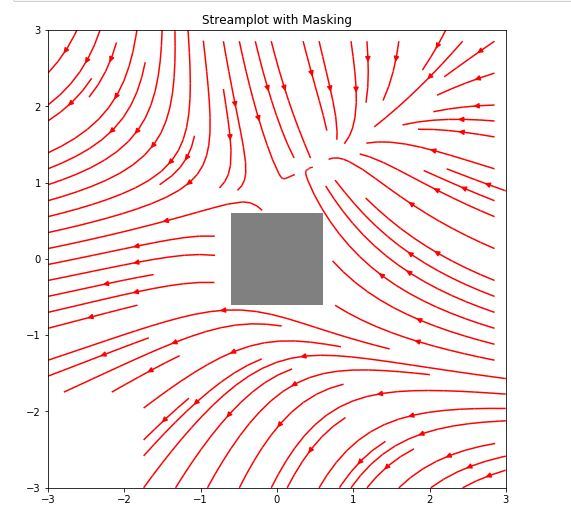
Streamlines skipping masked regions and NaN values –

Python3

# Import libraries
import numpy as np
import matplotlib.pyplot as plt
import matplotlib.gridspec as gridspec

# Creating dataset
w = 3
Y, X = np.mgrid[-w:w:100j, -w:w:100j]
U = -1 - X**2 + Y
V = 1 + X - Y**2
speed = np.sqrt(U**2 + V**2)

fig = plt.figure(figsize =(20, 16))
gs = gridspec.GridSpec(nrows = 3, ncols = 2, height_ratios =[1, 1, 2])

# Create a mask
mask = np.zeros(U.shape, dtype = bool)
mask[40:60, 40:60] = True
U[:20, :20] = np.nan
U = np.ma.array(U, mask = mask)

ax = fig.add_subplot(gs[2:, :])
ax.streamplot(X, Y, U, V, color ='r')
ax.set_title('Streamplot with Masking')

ax.imshow(~mask, extent =(-w, w, -w, w), alpha = 0.5,
          interpolation ='nearest', cmap ='gray', aspect ='auto')
ax.set_aspect('equal')

# show plot
plt.tight_layout()
plt.show()

Output:

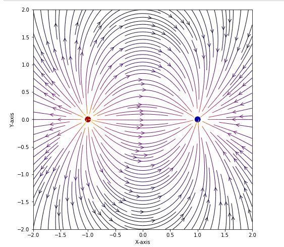
Example:
Stream plot to demonstrate the electric field due to two point charges.The electric field at any point on a surface depends upon the position and distance between the two charges:

Python3

import sys
import numpy as np
import matplotlib.pyplot as plt
from matplotlib.patches import Circle

# Function to determine electric field
def E(q, r0, x, y):
    den = np.hypot(x-r0[0], y-r0[1])**3
    return q * (x - r0[0]) / den, q * (y - r0[1]) / den

# Grid of x, y points
nx, ny = 64, 64
x = np.linspace(-2, 2, nx)
y = np.linspace(-2, 2, ny)
X, Y = np.meshgrid(x, y)

# Create a multipole with nq charges of
# alternating sign, equally spaced
# on the unit circle.

# Increase the power with increase in charge
nq = 2**1
charges = []
for i in range(nq):
    q = i % 2 * 2 - 1
    charges.append((q, (np.cos(2 * np.pi * i / nq),
                        np.sin(2 * np.pi * i / nq))))

# Electric field vector, E =(Ex, Ey)
# as separate components
Ex, Ey = np.zeros((ny, nx)), np.zeros((ny, nx))

for charge in charges:
    ex, ey = E(*charge, x = X, y = Y)
    Ex += ex
    Ey += ey

fig = plt.figure(figsize =(18, 8))
ax = fig.add_subplot(111)

# Plotting the streamlines with
# proper color and arrow
color = 2 * np.log(np.hypot(Ex, Ey))
ax.streamplot(x, y, Ex, Ey, color = color,
              linewidth = 1, cmap = plt.cm.inferno,
              density = 2, arrowstyle ='->',
              arrowsize = 1.5)

# Add filled circles for the charges
# themselves
charge_colors = {True: '#AA0000',
                 False: '#0000AA'}

for q, pos in charges:
    ax.add_artist(Circle(pos, 0.05,
                         color = charge_colors[q>0]))

ax.set_xlabel('X-axis')
ax.set_ylabel('X-axis')
ax.set_xlim(-2, 2)
ax.set_ylim(-2, 2)
ax.set_aspect('equal')

plt.show()

Output: