M-CTC-T Model in NLP

Automatic Speech Recognition (ASR) stands at the forefront of cutting-edge Natural Language Processing (NLP) applications, revolutionizing the way computers interact with spoken language. In this article, we embark on a journey to unravel the intricacies of an advanced ASR model known as M-CTC-T. This model, rooted in the principles of Connectionist Temporal Classification (CTC) and Transformer architecture, exemplifies the fusion of simplicity and sophistication. As we delve into its architecture, training methodology, and a unique fine-tuning approach involving pseudo-labeling, readers will gain insights into the inner workings of a state-of-the-art ASR solution.

Automatic Speech recognition

The Automatic Speech Recognition (ASR) system transcribes speech audio recordings into text. The input is audio, and the output is text.

The ASR model can be of two types:

1. CTC (Connectionist Temporal Classification): These are encoder-only models that take the input features of audio, transform the input into a hidden state, and use a CTC head on top to predict the text. Encoders are simpler models as compared to Seq2Seq, but one downside is that they tend to predict the character for each input feature, thereby requiring that the input and output have the same length, which will not be true for our ASR tasks. This is where CTC helps in the realignment of input and output by allowing the model to predict the same character multiple times. Wav2Vec2 and M-CTC-T are examples of such architecture.
2. Seq2Seq (Sequence to Sequence Models):models, These are encoder and decoder models allowing for different lengths of inputs and outputs as the input is processed by the encoder and the output is processed by the decoder. However, this model is complex and slower as compared to the CTC model.

This article assumes that the reader has a basic understanding of the below

1. How raw audio forms are converted into MEL spectrogram which are input for the ASR task.
2. Transformer architecture and self-attention mechanism.
3. Basics of deep learning – Conv1d, Binary layers, etc.

M-CTC-T Model

The M-CTC-T is a multilingual model i.e. a single model can transcribe the audio in all the 60 languages it was trained. It is a 1 Billion parameter model.

M-CTC-T Model Architecture

Below is the model architecture of the M-CTC-T model

M-CTC-T Model

For the M-CTC-T-Large model below are the main components along with their dimensions:

1. INPUT – The input to the encoder is a sequence of 80-dimensional log mel filterbank frames, extracted using 25 ms Hamming windows every 10ms from the 16 kHz audio signal. The maximum sequence length is 920
2. CONV 1D – There is a single gated convolution layer (CONV1d + GLU)which performs convolution along the time axis(1D). This takes 80 input features of the log mel spectrum and convert it to a 3072 output feature. The filter length is 7 and it has a stride of 3 with valid padding. The original paper had only one convolution layer. However the hugging face implementation has option of specifying multiple CONV layer through the config parameter ‘num_conv_layers’. GLU halves the output features- Given a tensor, we do two independent convolutions and get two output . We do sigmoid activation for one of the outputs. We then element-wise multiply the two outputs together. Thus the GLU halves the output features to 1536.
3. ENCODER – These consist of 36 layers of below :
   1. SELF ATTENTION – 4 heads of self-attention each of size 384. Thus the four attention combined take an input of 4*384 =1536 which is the output size of the convolution layer after GLU.
   2. INTERMEDIATE LAYER – The encoder output is feed to intermediate layer which is a linear layer that transforms the feature vector from 1536 to 6144.
   3. FEED FORWARD LAYER – The feedforward layer takes an input of 6144 and transforms it back to 1536. The final output of the encoder block is Batch * SeqLen * 1536
4. CTC Head – The CTC head is a linear layer with 8065 outputs. One for each character of all the 60 languages. including punctuation, space, and the CTC blank symbol.
5. LID Head – The Lid head is a linear layer with 60 outputs – one for each language followed by mean pooling to aggregate along the sequence length. These LID outputs are used only during training.

M-CTC-T Model Training

The objective of the author while developing the M-CTC-T model was to demonstrate the use of pseudo-labeling for multilingual ASR tasks.

What is Pseudo labelling?

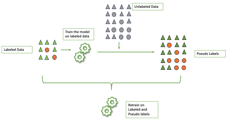
Pseudo-labeling is a semi-supervised technique that is used when we want to use unlabeled data. It is useful when we have a small set of labeled data along with a large set of unlabeled data. In pseudo labelling we keep adding add Pseudo-labeling in general consists of below steps:

1. INITIAL TRAINING : Train a initial baseline model on the available labelled data set
2. PREDICTIONS ON UNLABELED DATA : Use the model obtained in Step 1 to predict labels of the unlabeled datasets. These are know as Pseudo Labels (PL).
3. AUGMENT TRAINING DATASET : The pseudo labels generated is combined with the initial labeled data set used for generating baseline model. Here one can also include only those pseudo labels to be included which has a high prediction score/confidence.
4. RETRAINING: Now either retrain the same model or train a new model from scratch on the pseudo labels and labeled dataset combined.
5. ITERATIONS : Steps 2 to 4 can be repeated to improve model robustness.

One must be careful in using this technique as too many of noisy sample in Pseudo labels will negatively impact the model performance. However this technique has shown to improve performance in ASR task considerably and gained momentum especially in speech related task.

Pseudo Label Process

The above is a general approach and many variants exist. For the ASR task the author adopted the below process

1. There are two open source data available for the ASR task-
   • CV (Common Voice) which is labelled and consists of samples from 60 languages
   • VP (Vox Populli) which is unlabeled and consists of samples from 23 languages. 19 languages are common between CV and VP dataset.
2. The author of the M-CTC-T model followed a technique which is based on sLimIPL (Language-Model-Free Iterative Pseudo-Labeling) developed by the Facebook .
3. The author first trained a model for several updates on labeled data of the CV dataset. After this step, the multilingual model is obtained.
4. Then the model was first fine tuned for a particular language for which pseudo label had to be generated. This fine-tuned model generated pseudo labels of the VP dataset for the language in which it was trained. In total 19 slimIPL models were developed to generate PLs for the 19 languages that were common between the CV and VP dataset.
5. The PL of all languages were pooled together along with the labelled data of CV and a new model was trained from scratch. The author found it that training a new model from scratch yielded better results then training the the non-fine-tuned multilingual model checkpoint (model obtained after step 3 before running slimIPL).

Automatic Speech recognition

M-CTC-T Model Implementations

Below is the code for inference and fine tuning of M-CTC-T large model.

Install and Import Necessary Libraries

The google notebook is here

Install the below libraries if not available in your environment. These are required to run the subsequent code.

• Torch is an open source ml framework that provides flexible an efficient platform for building and training deep neural networks
• Dataset is required for loading the data on which we will finetune or model.
• Transformers is required to load the pretrained model from hugging face
• transformers[batch] contains libraries required that is required while fine tuning like accelerate
• Jiwer is required for model evaluation

!pip install datasets
!pip install transformers
!pip install torch
!pip install evaluate
!pip install jiwer
!pip install transformers[torch]

And then import the libraries into your notebook

Python3

#Imports required
import numpy as np
from datasets import load_dataset, Audio
from transformers import MCTCTProcessor, MCTCTForCTC
import torch
import evaluate
from dataclasses import dataclass, field
from typing import Any, Dict, List, Optional, Union
from transformers import TrainingArguments, Trainer

Loading Dataset and Preprocessing

Using the load_dataset function of datasets library we load the minds14 dataset in ‘English’ from hugging face. We load only 80 samples for our demo purpose .

About the PloyAi/minds14 dataset- MINDS-14 is training and evaluation resource for intent detection task with spoken data. It covers 14 intents extracted from a commercial system in the e-banking domain, associated with spoken examples in 14 diverse language varieties

Data Fields

1. path (str): Path to the audio file
2. audio (dict): Audio object including loaded audio array, sampling rate and path ot audio
3. transcription (str): Transcription of the audio file
4. english_transcription (str): English transcription of the audio file
5. intent_class (int): Class id of intent
6. lang_id (int): Id of language

We remove the unnecessary colunms using remove_columns method on dataset

We then split the dataset in ration of 80: 20. We specify shuffle= false so that we get same example while running the code

Python3

# Load the PolyAI dataset.
dataset = load_dataset("PolyAI/minds14", name="en-US", split="train[:80]")

# Remove unnecessary columns
dataset = dataset.remove_columns(['path','english_transcription','intent_class'])

# Split the dataset into train and test
dataset = dataset.train_test_split(test_size = 0.2, shuffle=False)

Resampling data

We need to resample the data to 16khz as the M-CTC-T model is trained in 16khz and the dataset is in 8khz. For this we make use of the Audio library.

Python3

# Declare device variable
device = 'cuda' if torch.cuda.is_available() else'cpu'

# Resample the dataset to 16 Khz as MCTCT model is trained on 16khz
dataset = dataset.cast_column("audio", Audio(sampling_rate=16000))

Loading Pretrained model

We will be loading the pretrained model from hugging face.

The model has been contributed by Speechbrain. The model is a 1B-param transformer encoder, with a CTC head over 8065 character labels and a language identification head over 60 language ID labels. The Auto processor is a wrapper of feature extractor and tokenizer required for M-CTC-T model. The purpose of feature extractor is to processes the speech signal to the model’s input format, e.g. a feature vector, and the tokenizer processes the model’s output format to text. We will initialize autoprocessor and pass our input dataset obtained from above step to it.

Python3

# Loading the model and autoprocessor  from transformer
# Autoprocessor is a wrapper of feature extractor and tokenizer

processor = MCTCTProcessor.from_pretrained("speechbrain/m-ctc-t-large")
model = MCTCTForCTC.from_pretrained("speechbrain/m-ctc-t-large")
model.to(device)

Drawing Inferences

Let us format one of the input and infer its transcription using the mase model. The model gives output in logits. We take the max of the logits and decode it.

The torch.no_grad() section indicates the operations should not be included in gradient computation, which is useful when you don’t need to update model weights.

Python3

# Lets process the first example of train dataset

inputs = processor(dataset['train'][3]["audio"]["array"], sampling_rate=16000, return_tensors="pt")

# getting the predictions

with torch.no_grad():
    logits = model(**inputs).logits


predicted_ids = torch.argmax(logits, dim=-1)
transcription = processor.batch_decode(predicted_ids)
transcription

Output:

['How do wy started to an account?']

The actual text of the audio is ‘how do I start a joint account’ .

Let us fine-tuning the model to get a better output using the below steps.

Fine Tuning the model

We need to preprocess the data as per the format expected by the M-CTC-T model. We do so by using the Dataset map function

We need to create two columns with name ‘input_featrues'(input array of sound wave in raw form needs to be resampled to 16khz and feature extracted in the log mel filterbank frames) and ‘labels'(transcription as per the tokenizer format). This is done by passing each data to the processor defined above .

Python3

# Preparing a function to process the entire dataset

def prepare_dataset(batch):
    audio = batch["audio"]

    batch["input_features"] = processor(audio["array"], sampling_rate=audio["sampling_rate"]).input_features[0]

    with processor.as_target_processor():
        batch["labels"] = processor(batch["transcription"]).input_ids
    return batch

encoded_dataset = dataset.map(prepare_dataset, num_proc=4)

Creating a Specialised class for Data

Let’s create a DataCollator Class specifically for fine-tuning MCTCT, as the Transformer models do not inherently provide a data collator for Automatic Speech Recognition (ASR). To achieve this, we’ll adapt the DataCollatorWithPadding class to generate batches of examples. These examples consist of elements of the same type as those found in the train_dataset or eval_dataset.

It’s crucial to note that input_features and labels require different padding strategies since they may have varying lengths. This distinction is essential because in ASR, input and output are distinct modalities and should not be subjected to the same padding function. Given the potentially large input sizes in ASR tasks, it is more efficient to dynamically pad training batches. This means that each training sample should only be padded to match the length of the longest sample within its batch, rather than padding to the overall longest sample. The DataCollator will handle this dynamic padding during the training process.

In summary, for fine-tuning MCTCT, we need a specialized padding data collator, which we will define below:

Python3

from dataclasses import dataclass, field
from typing import Any, Dict, List, Optional, Union


@dataclass
class DataCollatorCTCWithPadding:
    processor: MCTCTProcessor
    padding: Union[bool, str] = "longest"

    def __call__(self, features: List[Dict[str, Union[List[int], torch.Tensor]]]) -> Dict[str, torch.Tensor]:
        # split inputs and labels since they have to be of different lengths and need
        # different padding methods
        input_features = [{"input_features": feature["input_features"]} for feature in features]
        label_features = [{"input_ids": feature["labels"]} for feature in features]

        batch = self.processor.pad(input_features, padding=self.padding, return_tensors="pt")

        labels_batch = self.processor.pad(labels=label_features, padding=self.padding, return_tensors="pt")

        # replace padding with -100 to ignore loss correctly
        labels = labels_batch["input_ids"].masked_fill(labels_batch.attention_mask.ne(1), -100)

        batch["labels"] = labels

        return batch

data_collator = DataCollatorCTCWithPadding(processor=processor, padding="longest")

Evaluation Metric

For our task we will be using the word error rate metric. We should define a compute_metrics function accordingly

The model will produce a series of logit vectors, each of which comprises log-odds for every word in the previously established vocabulary. In other words, the length of each logit vector equals the configured vocabulary size, denoted as config.vocab_size. Our primary concern lies in determining the most probable prediction generated by the model, which is achieved by calculating the argmax(…) of the logits. Additionally, we convert the encoded labels back into their original string form. This process involves replacing instances of -100 with the pad_token_id and decoding the IDs while ensuring that consecutive tokens are not incorrectly grouped together in a manner consistent with the CTC (Connectionist Temporal Classification) style. Finally, we compare the decoded output with the ground truth to calculate the error rate.

Python3

# Getting the evaluation metrics
wer = evaluate.load("wer")

# Defining the metrics functions
def compute_metrics(pred):
    pred_logits = pred.predictions
    pred_ids = np.argmax(pred_logits, axis=-1)

    pred.label_ids[pred.label_ids == -100] = processor.tokenizer.pad_token_id

    pred_str = processor.batch_decode(pred_ids)
    label_str = processor.batch_decode(pred.label_ids, group_tokens=False)

    wer = wer.compute(predictions=pred_str, references=label_str)

    return {"wer": wer}

Model Training

In a final step, we define all parameters related to training. To give more explanation on some of the parameters:

• learning_rate (float, optional, defaults to 5e-5) — The initial learning rate for the optimizer.
• group_by_length makes training more efficient by grouping training samples of similar input length into one batch.
• gradient checkpointing– enables saving a lot of GPU memory
• fp_16 – Whether to use float point 16 precision instead of standard 32 bit precision. this helps in saving memory
• per_device_train_batch_size (int, optional, defaults to 8) — The batch size per GPU/XPU/TPU/MPS/NPU core/CPU for training.
• per_device_eval_batch_size (int, optional, defaults to 8) — The batch size per GPU/XPU/TPU/MPS/NPU core/CPU for evaluation.
• We use optim=’adafactor’ as it offers better memory management

Note – Since its a large model it takes significant amount of memory. Its requires GPU for training. If enough memory is not available one may encounter out of memory issues. Learning_rate was heuristically tuned until fine-tuning has become stable. Note that those parameters strongly depend on the dataset and one must try with different values for different dataset

Pass the above training arguments to Trainer along with dataset, model, tokenizer, data collator and call .train() on it to start the training.

Python3

del model
model = MCTCTForCTC.from_pretrained('speechbrain/m-ctc-t-large',ctc_loss_reduction="mean",pad_token_id=processor.tokenizer.pad_token_id)
model.to(device)

# defining training arguments and trainer
training_args = TrainingArguments(
    output_dir="m-ctc-t_trained",
    gradient_checkpointing=True,
    per_device_train_batch_size=1,
    learning_rate=1e-5,
    warmup_steps=2,
    max_steps=2000,
    fp16=True,
    optim='adafactor',
    group_by_length=True,
    evaluation_strategy="steps",
    per_device_eval_batch_size=1,
    eval_steps=100,
    load_best_model_at_end=True,
    metric_for_best_model="wer",

)

trainer = Trainer(
    model=model,
    args=training_args,
    train_dataset=encoded_dataset["train"],
    eval_dataset=encoded_dataset["test"],
    tokenizer=processor.feature_extractor,
    data_collator=data_collator,
    compute_metrics=compute_metrics,
)

trainer.train()

Output:

Step    Training Loss    Validation Loss    Wer
100    No log    1.023276    0.467742
200    No log    1.218436    0.435484
300    No log    1.160553    0.443548
400    No log    1.444840    0.435484
500    3.066700    1.962108    0.403226
600    3.066700    2.487072    0.403226
700    3.066700    2.188133    0.435484
800    3.066700    2.187747    0.459677

Getting Prediction from the Fine tuned model

With the model now trained, we will get a prediction from the dataset.

Python3

## getting test data
i2 = processor(dataset['test'][6]["audio"]["array"], sampling_rate=16000, return_tensors="pt")
print(f"The input test audio is: {dataset['test'][6]['transcription']}")

# prediction for test data
with torch.no_grad():
    logits = model(**i2.to(device)).logits

predicted_ids = torch.argmax(logits, dim=-1)
transcription = processor.batch_decode(predicted_ids)
print(f'The output prediction is : {transcription[0]}')

Output:

The input test audio is: so you spent the money I'd like to see my new account balance
The output prediction is : so I just spent some money I'd like to see my new account balance

We can save the model using trainer.save_model(“path_to_save”). Latter you can load the model from the saved path directly use for interference.

Conclusion

In the rapidly evolving landscape of Natural Language Processing, the significance of Automatic Speech Recognition cannot be overstated. The M-CTC-T model, with its multilingual capabilities and one billion parameters, epitomizes the prowess of modern ASR systems. From the initial preprocessing of raw audio to the intricacies of its Transformer architecture, we’ve navigated through the core components of this model.

A key highlight of this article lies in the exploration of pseudo-labeling, a semi-supervised technique that leverages unlabeled data to enhance the robustness of the ASR model.