How to Train Tensorflow Models in Python

TensorFlow is a popular open-source machine learning framework that allows you to build, train, and deploy deep learning models. It provides a wide range of tools and functionalities for developing powerful neural networks. In this article, we will explore the process of training TensorFlow models in Python.

Let us see some basic steps needed to train a TensorFlow model:

Install TensorFlow

Before we begin, make sure you have TensorFlow installed on your system. You can use pip, the Python package manager, to install TensorFlow by running the following command in your terminal:

pip install tensorflow

Step 1: Import the required Libraries:

Once TensorFlow is installed, you need to import the required libraries into your Python script. Along with TensorFlow, you may also need to import other libraries for data preprocessing, visualization, or evaluation. Here’s an example of importing TensorFlow and Numpy:

Python

import tensorflow as tf
import numpy as np
import tensorflow_datasets as tfds
import matplotlib.pyplot as plt

Step 2: Load & Prepare the Dataset:

Before training a TensorFlow model, you need to load & prepare our dataset. This involves the following tasks:

• Load the dataset
• Data cleaning,
• Preprocessing,
• Normalization and
• Splitting into training and validation sets.

You should also consider converting your data into a format that TensorFlow can efficiently work with, such as NumPy arrays or TensorFlow Datasets.

Load the dataset

The CIFAR-10 dataset is a commonly used benchmark dataset in computer vision. It consists of 60,000 color images, each of size 32×32 pixels, belonging to 10 different classes. The dataset is split into 50,000 training images and 10,000 test images.

• I use the tfds.load() function to load the CIFAR-10 dataset.
• I specify the split argument to get the training and test splits of the dataset.
• Additionally, with_info=True allows us to retrieve information about the dataset, including the number of classes.

Python3

# Load data
dataset_name = 'cifar10'
(train_dataset, test_dataset), dataset_info = tfds.load(name=dataset_name,
                                                       split=['train', 'test'],
                                                       shuffle_files=True,
                                                       with_info=True,
                                                       as_supervised=True)

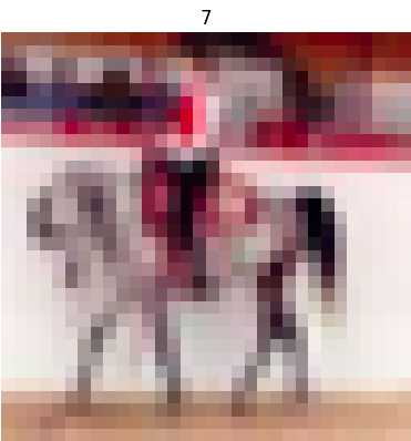
Plot an image from the dataset

Python3

image, label = next(iter(train_dataset.take(1)))

plt.imshow(image)
plt.title(label.numpy())
plt.axis('off')
plt.show()

Output:

Get the number of classes in the dataset

Python3

# Get the number of classes in the dataset
num_classes = dataset_info.features['label'].num_classes
num_classes

Output:

10

Preprocessing & Normalization

Define a preprocessing function preprocess_data() that converts the images to float32 and normalizes their values between 0 and 1.

Python3

# Preprocess the data
def preprocess_data(image, label):
    # Convert image to float32 and normalize between 0 and 1
    image = tf.cast(image, tf.float32) / 255.0
    return image, label

Apply this preprocessing function to both the training and test datasets.

Python3

# Apply preprocessing to the datasets
train_dataset = train_dataset.map(preprocess_data)
test_dataset = test_dataset.map(preprocess_data)

Step 3: Build Your Model

The next step is to define the architecture of your TensorFlow model. TensorFlow provides various APIs for model building, such as the Sequential API and the Functional API. You can choose the one that best suits your needs. Specify the layers, activation functions, loss function, and optimizer for your model.

In terms of model architecture, the convolutional layers (Conv2D) apply a set of filters to the input image, extracting different features at each layer. The max-pooling layers (MaxPooling2D) reduce the spatial dimensions of the feature maps. The dense layers (Dense) are fully connected layers that connect all the neurons from the previous layer to the current layer. The ReLU activation function (relu) introduces non-linearity to the model, allowing it to learn complex relationships. The final dense layer with softmax activation outputs a probability distribution over the classes.

• The model here build is a convolutional neural network (CNN) using the Sequential API from tf.keras.
• It consists of three convolutional layers with increasing numbers of filters, followed by max-pooling layers to downsample the feature maps.
• Then, Flatten the output and add two fully connected layers (dense layers) with ReLU activation functions.
• The final dense layer has a softmax activation function to output the probabilities for each class.
• The summary() method is called on the model to print a summary of the model architecture.
• The model summary provides information about each layer, its output shape, and the number of parameters.

Python

# Step 3: Build the model
input_dim = (32, 32, 3)

model = tf.keras.models.Sequential([
    tf.keras.layers.Conv2D(32, (3, 3), activation='relu', input_shape=input_dim),
    tf.keras.layers.MaxPooling2D((2, 2)),
    tf.keras.layers.Conv2D(64, (3, 3), activation='relu'),
    tf.keras.layers.MaxPooling2D((2, 2)),
    tf.keras.layers.Conv2D(64, (3, 3), activation='relu'),
    tf.keras.layers.Flatten(),
    tf.keras.layers.Dense(64, activation='relu'),
    tf.keras.layers.Dense(num_classes, activation='softmax')
])
# Print the model summary
model.summary()

Output:

Model: "sequential"
_________________________________________________________________
 Layer (type)                Output Shape              Param #   
=================================================================
 conv2d (Conv2D)             (None, 30, 30, 32)        896       
                                                                 
 max_pooling2d (MaxPooling2D  (None, 15, 15, 32)       0         
 )                                                               
                                                                 
 conv2d_1 (Conv2D)           (None, 13, 13, 64)        18496     
                                                                 
 max_pooling2d_1 (MaxPooling  (None, 6, 6, 64)         0         
 2D)                                                             
                                                                 
 conv2d_2 (Conv2D)           (None, 4, 4, 64)          36928     
                                                                 
 flatten (Flatten)           (None, 1024)              0         
                                                                 
 dense (Dense)               (None, 64)                65600     
                                                                 
 dense_1 (Dense)             (None, 10)                650       
                                                                 
=================================================================
Total params: 122,570
Trainable params: 122,570
Non-trainable params: 0
_________________________________________________________________

Generate the model graph

To plot the model graph, graphviz and pydot should be installed in the system

sudo apt install graphviz  # For Ubuntu
pip install pydot

• The plot_model() function from tf.keras.utils is used to generate a graphical visualization of the model.
• The show_shapes=True argument ensures that the shapes of the input and output tensors of each layer are displayed in the graph.

Python3

#Generate the model graph
tf.keras.utils.plot_model(model, show_shapes=True)

Output:

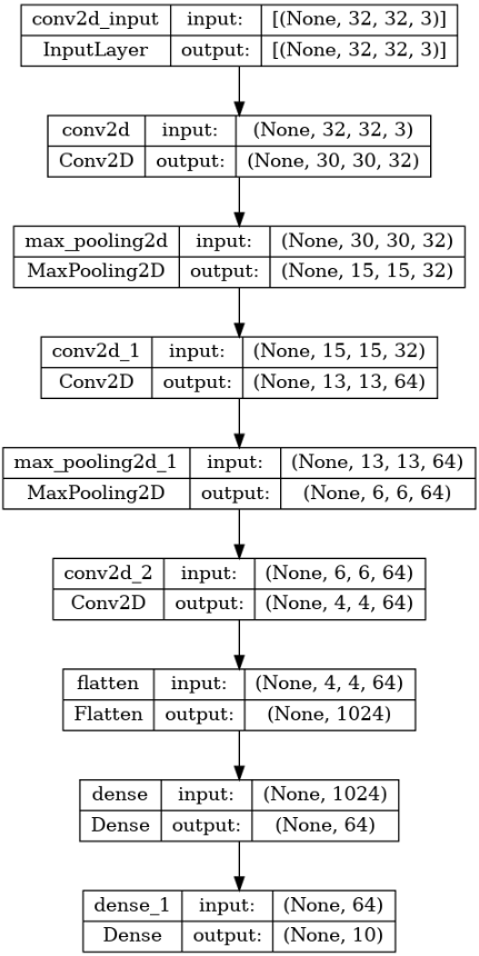
Now, Let’s go through each layer in the model:

1. Conv2D layer: This layer performs convolutional operations on the input data. In the CIFAR-10 example, the first Conv2D layer has 32 filters of size 3×3. Convolution involves sliding these filters over the input image and computing dot products between the filter weights and the corresponding image patches. This helps extract different features from the input image.
2. MaxPooling2D layer: The MaxPooling2D layer downsamples the feature maps obtained from the previous convolutional layers. It reduces the spatial dimensions by taking the maximum value within a given window (2×2) and moving it across the input. This helps reduce the number of parameters in the model and captures the most salient features.
3. Flatten layer: The Flatten layer flattens the multidimensional feature maps into a 1D vector. This is required to connect the convolutional layers to the subsequent fully connected (dense) layers.
4. Dense layers: The Dense layers are fully connected layers. The first dense layer has 64 units and uses the ReLU activation function. It takes the flattened features from the previous layer as input and learns complex representations by applying weights and biases to the input data. The second dense layer has num_classes (in this case, 10) units, representing the output classes of the dataset. It uses the softmax activation function to produce a probability distribution over the classes.

Step 4: Compile the Model

After building your model, you need to compile it by specifying the optimizer, loss function, and any additional metrics you want to track during training. The optimizer determines the algorithm used to update the model’s parameters during training.

• compile the model using the compile() method. This step configures the model for training by specifying the optimizer and loss function. Additionally, we can specify metrics to evaluate during training, such as accuracy.
• Specify the optimizer as ‘adam‘, which is a popular optimization algorithm.
• The loss function is set to SparseCategoricalCrossentropy, It is a multi-class classification tasks. It compares the predicted class probabilities with the true labels and computes the loss. I set from_logits=True it because the last layer of our model does not have a softmax activation applied directly.

Python

#Compile the model
model.compile(optimizer='adam',
              loss=tf.keras.losses.SparseCategoricalCrossentropy(from_logits=True),
              metrics=['accuracy'])

Step 5: Train the Model

With the model compiled, you can now train it using your prepared data. Pass the training data and labels to the fit function along with the desired number of epochs (iterations over the dataset). During training, the model will adjust its weights and biases to minimize the defined loss function.

• Decide the hyperparameter like the number of batches and number of epochs
• Map the dataset into batches
• The fit() method is used to train the model. It takes the training dataset as input and iteratively updates the model’s weights. During training, the model makes predictions on the input data, computes the loss based on the predicted values and true labels, and propagates the gradients backward through the network using back-propagation. The optimizer then adjusts the weights based on the gradients to minimize the loss.

Python

batch_size = 128
num_epochs = 10
# To process the dataset in batches create the batches of batch_size
train_dataset = train_dataset.batch(batch_size).prefetch(tf.data.AUTOTUNE)
test_dataset = test_dataset.batch(batch_size)

#Train the model
model.fit(train_dataset, epochs=num_epochs, validation_data=test_dataset)

Output:

Epoch 1/10
391/391 [==============================] - ETA: 0s - loss: 1.6713 - accuracy: 0.3879
391/391 [==============================] - 16s 39ms/step - loss: 1.6713 - accuracy: 0.3879 - val_loss: 1.4350 - val_accuracy: 0.4811
Epoch 2/10
391/391 [==============================] - 14s 37ms/step - loss: 1.3312 - accuracy: 0.5247 - val_loss: 1.2660 - val_accuracy: 0.5524
Epoch 3/10
391/391 [==============================] - 14s 36ms/step - loss: 1.1847 - accuracy: 0.5815 - val_loss: 1.1334 - val_accuracy: 0.5991
Epoch 4/10
391/391 [==============================] - 14s 36ms/step - loss: 1.0878 - accuracy: 0.6194 - val_loss: 1.0829 - val_accuracy: 0.6184
Epoch 5/10
391/391 [==============================] - 14s 35ms/step - loss: 1.0198 - accuracy: 0.6441 - val_loss: 1.0434 - val_accuracy: 0.6356
Epoch 6/10
391/391 [==============================] - 13s 34ms/step - loss: 0.9628 - accuracy: 0.6676 - val_loss: 1.0030 - val_accuracy: 0.6527
Epoch 7/10
391/391 [==============================] - 14s 35ms/step - loss: 0.9128 - accuracy: 0.6840 - val_loss: 0.9670 - val_accuracy: 0.6617
Epoch 8/10
391/391 [==============================] - 14s 35ms/step - loss: 0.8685 - accuracy: 0.6990 - val_loss: 0.9345 - val_accuracy: 0.6732
Epoch 9/10
391/391 [==============================] - 13s 34ms/step - loss: 0.8306 - accuracy: 0.7118 - val_loss: 0.9152 - val_accuracy: 0.6831
Epoch 10/10
391/391 [==============================] - 14s 37ms/step - loss: 0.7995 - accuracy: 0.7223 - val_loss: 0.9030 - val_accuracy: 0.6859

Step 6: Evaluate the Model

Once the model is trained, you can evaluate its performance using the validation or test data. This will provide insights into its accuracy, loss, and any other metrics you defined. The evaluation methods return the test loss and any other specified metrics.

Python

# Step 7: Evaluate the model
loss, accuracy = model.evaluate(test_dataset)
print("Test loss:", loss)
print("Test accuracy:", accuracy)

Output:

79/79 [==============================] - 1s 14ms/step - loss: 0.9030 - accuracy: 0.6859
Test loss: 0.9030246138572693
Test accuracy: 0.6858999729156494

Step 8: Make Predictions

After training and evaluating the model, you can use it to make predictions on new, unseen data. The predict method takes input data and returns the model’s predictions.

Python

# create a custom array of image size
new_image = tf.constant(np.random.rand(32, 32, 3), dtype=tf.float64)
# Extend the dimension 4D
new_image = tf.expand_dims(new_image, axis=0)

# Prediction
predictions = model.predict(new_image)
# predicted label
pred_label = tf.argmax(predictions, axis =1)
pred_label.numpy()

Output:

1/1 [==============================] - 0s 15ms/step
array([6])