How to export two HTML widgets in the same HTML page in R?

HTML widgets are interactive web components that can be embedded within an HTML document. They are created using R packages that provide bindings to JavaScript libraries. HTML widgets allow us to create dynamic and interactive visualizations, charts, maps, and others directly from R Programming Language.
In order to install it, type the following in the R console and press Enter and perform the necessary:-

install.packages("htmlwidgets")

The htmlwidgets package in R serves as a framework for creating R bindings to JavaScript libraries. It enables the creation of HTML widgets that can be used in multiple scenarios they can be used interactively in the R console similar to traditional R plots, can be seamlessly embedded within R Markdown documents, incorporated into Shiny web applications, saved as standalone web pages, and others.

When analyzing and presenting data, it is often helpful to provide multiple related visualizations together. Hence by exporting multiple HTML widgets into a single HTML file, we can provide a comprehensive view of the data. So we try to perform the same using HTML widgets in R programming language.

For this, we will consider two simple widgets made using one of the popular HTML widgets plotly. If not installed, install it via the following command:-

install.packages("plotly")

Plotly is an R package that provides an interface to the Plotly.js JavaScript library, allowing users to create interactive and dynamic visualizations directly from R. Plotly supports a wide range of chart types, including scatter plots, line plots, bar charts, histograms, heatmaps, and more. It is popular due to its versatility, interactivity, and most important its ability to handle large datasets easily.
Post-installation we can create two simple widgets:-

R

library(plotly)

# Create the first plotly widget
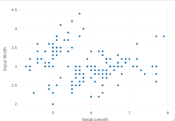
widget1 <- plot_ly(data = iris, x = ~Sepal.Length, y = ~Sepal.Width, type = "scatter",
                   mode = "markers")

# Create the second plotly widget
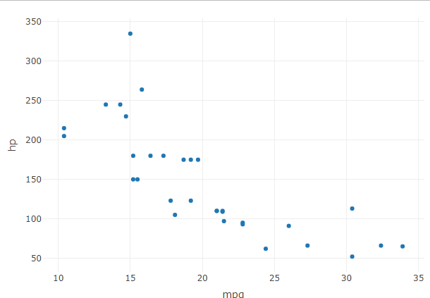
widget2 <- plot_ly(data = mtcars, x = ~mpg, y = ~hp, type = "scatter",
                   mode = "markers")

widget1
widget2

Output:

Export two HTML widgets in the same HTML page in R

In the code snippet iris and mtcars are names of datasets that come preloaded with R.

Export two HTML widgets in the same HTML page in R

1. iris: The iris dataset is a classic dataset in statistics and is often used for data analysis and visualization. It contains measurements of four attributes (sepal length, sepal width, petal length, and petal width) for three different species of iris flowers (setosa, versicolor, and virginica). Each row in the dataset represents an individual iris flower, and the columns represent the different attributes.
2. mtcars: The mtcars dataset is another commonly used dataset in R, which contains information about various car models and their performance characteristics. It includes data such as miles per gallon (mpg), horsepower (hp), and other variables related to car specifications. Each row represents a different car model, and the columns represent different variables.

In the code snippet, the plot_ly() function is used to create scatter plots based on these datasets. For widget1, the scatter plot is created using the iris dataset, specifically using the Sepal.Length variable as the x-axis and the Sepal.Width variable as the y-axis. Similarly, for widget2, the scatter plot is created using the mtcars dataset, with mpg as the x-axis and hp as the y-axis.

The type parameter in plot_ly() function determines the overall visualization or chart type like scatter plots, bar plots, line plots, etc. Here type = "scatter" indicates that a scatter plot should be created. The mode parameter defines how the data points are displayed within the plot and include options like markers, lines, or text labels. In above code mode = "markers" specifies that the data points should be displayed as markers on the scatter plot.

Now lets visualize how the interactive plots actually look like. We can use the htmlwidgets::saveWidget() function to save the plotly widgets as standalone HTML files and open them in a web browser after execution of the below R file.

R

library(plotly)
library(htmlwidgets)

# Create the first plotly widget
widget1 <- plot_ly(data = iris, x = ~Sepal.Length, y = ~Sepal.Width, type = "scatter", mode = "markers")

# Create the second plotly widget
widget2 <- plot_ly(data = mtcars, x = ~mpg, y = ~hp, type = "scatter", mode = "markers")

# Save the widgets as standalone HTML files
saveWidget(widget1, "widget1.html")
saveWidget(widget2, "widget2.html")

Output:

Export two HTML widgets in the same HTML page in R

In order to execute the above code save it as some filename with a `.r` extension (i.e. filename. r). Then in the terminal simply type.
Wait for the code to execute completely, after it finishes notice that two html files will be generated in the present working directory named as widget1.html and widget2.html. Now open them in the browser to view them.

Rendering the above two HTML widgets on the same HTML page

To render the two widgets in a single HTML page , we utilize the R Markdown fileWe utilize the R Markdown file to render the two widgets in a single HTML page. When we render the R Markdown file, it executes the code page chunks, generates the HTML output, and incorporates the rendered HTML widgets into the resulting HTML file. This approach enables us to embed multiple interactive HTML widgets within a single HTML document.

When we render an R Markdown file, Pandoc is invoked behind the scenes to convert the Markdown content, code chunks, and outputs into the final output format.

Pandoc is a separate software that needs to be installed on your system in order to work with R Markdown. Pandoc is a powerful document converter and a key component in the R Markdown ecosystem. It is a command-line tool that allows us to convert documents from one format to another. It supports a wide range of input and output formats, including HTML, PDF, Word documents, Markdown, and more. Pandoc converts the R Markdown content, code chunks, and outputs into the final output format specified in the YAML header of the R Markdown document. Please install it as it will be required in our R markdown file.

Steps to create R markdown file(.Rmd)

An R Markdown file is a plain text file with the extension .Rmd that combines narrative text, code, and output into a single document. It allows you to create dynamic reports, presentations, and dashboards by integrating R code and its results with explanatory text written in Markdown. If you are familiar with Python programming language and Jupyter Notebook (.ipynb) files the R markdown file structure might look similar though they are not the same. It basically has 3 main parts:-

The YAML Header – YAML (YAML Ain’t Markup Language) header is a section at the beginning of the document enclosed by --- (three dashes) that contains metadata and options for rendering the document. It is written in YAML syntax, which is a human-readable data serialization format. Common fields in the YAML header include title, author, date, and output.

Please don’t even skip a line at start of the R markdown file else the YAML header won’t get recognized causing a error in compilation. Hence the very first line of your R markdown file must contain `—`(3 dashes). See the below example.

---
title: "GFG's R Markdown Document"
author: "GFG author"
date: "2023-06-25"
output: html_document
---

Markdown Text – Following the YAML header, we can write narrative text using Markdown syntax. Markdown is a lightweight markup language that allows you to format text using simple and readable syntax.

# This is a H1 heading
This is a paragraph of text. Here's a bullet list:
- GeeksForGeeks : Your go-to platform for all questions
- Stuck on a problem? Don't worry, we've got you covered!
- Click on the link below to explore.
![visit_GFG](https://www.geeksforgeeks.org/)

R Code Chunks – R code chunks allow us to include and execute R code within the R Markdown document. Code chunks are enclosed within three backticks followed by {r} to indicate that it’s an R code chunk. We can specify additional options for code chunks, such as echo (whether to display the code), eval (whether to evaluate the code), and more. Then Click on ‘Run Chunk’ to run the code.

R

# Calculate the sum of two numbers
a <- 5
b <- 3
sum <- a + b
sum

Output:

[1] 8

Now let’s see an example of implementing two HTML widgets into a single html file in R markdown by following the below steps.

Create a YAML header

It contains metadata and options that specify how the R Markdown document should be rendered.

R

---
title: "Multiple HTMLWidgets in Single HTML Page"
output: html_document
---

• The title sets the title of the document that will appear in the rendered HTML output.If not provided defaults to title based on the filename of the R Markdown document.
• Specifying the output type is mandatory in the YAML header of an R Markdown document. The output field is used to define the desired output format for the rendered document.

Note:- If you omit the output field in the YAML header, an error will occur during the rendering process, and the document will fail to compile.

Code Chunk Setup and Options

In an R Markdown (.Rmd) file, the code enclosed within the back-ticks(`) is called a code chunk. Code chunks allow you to include and execute R code within your Rmd document.

R

```{r setup, include=FALSE}
knitr::opts_chunk$set(echo = TRUE)
library(plotly)

# Create the first plotly widget
widget1 <- plot_ly(data = iris, x = ~Sepal.Length, y = ~Sepal.Width,
                   type = "scatter", mode = "markers")

# Create the second plotly widget
widget2 <- plot_ly(data = mtcars, x = ~mpg, y = ~hp, type = "scatter",
                   mode = "markers")
```

• {r setup, include=FALSE} is the code chunk header. It specifies that this is an R code chunk and sets the chunk options. In this case, setup is the name of the chunk(can be named as user choice or left blank), and include=FALSE indicates that the code and its output should not be included in the rendered document.
• knitr::opts_chunk$set(echo = TRUE) sets an option for the code chunks in the document. knitr::opts_chunk refers to the options for code chunks, and $set(echo = TRUE) sets the option echo to TRUE. The echo option controls whether the code itself is displayed in the output document. Setting it to TRUE ensure that the code will be displayed. If you omit the line knitr::opts_chunk$set(echo = TRUE), the default behavior of code chunk display will be used, which is typically to show the code. Therefore, even without explicitly setting echo = TRUE, your code will still work fine and display the code within the code chunks.

Including the line knitr::opts_chunk$set(echo = TRUE) can be helpful if you want to ensure consistent behavior across multiple code chunks in your document. It allows you to set the code display option globally instead of specifying it individually for each code chunk.

When we use the Plotly package in R to create a widget, we don’t need to explicitly load or use the htmlwidgets package. The plotly package internally handles the conversion of Plotly charts into HTML widgets. The conversion to an HTML widget is still happening behind the scenes because of the integration between the plotly package and the htmlwidgets framework. This integration enables us to easily create interactive Plotly charts and embed them in various output formats, such as HTML documents, Shiny applications, and R Markdown files.

3. Calling Widgets in Code Chunk

R

```{r plotly}
widget1
widget2
```

• The {r} indicates that it is an R code chunk, and plotly is an optional label that can be used to name or identify the chunk. The label is useful when we want to refer to the specific chunk later in the document like when creating cross-references or executing code conditionally based on chunk labels. Including plotly as the chunk label does not have any specific meaning or functionality on its own. It is just a user-defined label.
• widget1 and widget2 are objects that represent Plotly widgets. widget1 is a scatter plot of the “Sepal. Length” variable on the x-axis and the “Sepal. Width” variable on the y-axis, using the “iris” dataset. widget2 is another scatter plot, using the “mpg” variable on the x-axis and the “hp” variable on the y-axis, using the “mtcars” dataset. These objects store the configuration and data for the respective Plotly widgets, and when executed, they are displayed as interactive plots in the R Markdown output.

4. Saving and executing the R Markdown file

We now need to save the R markdown as file as “filename.Rmd”. The entire code is given below for clarity and can be copied easily for testing purpose.

R

---
title: "Multiple HTMLWidgets in Single HTML Page"
output: html_document
---
<!-- save as  "filename.Rmd", html file will be generated in current location as file
with name as "filename.html" -->

<!-- setting up the widgets -->
```{r setup, include=FALSE}
knitr::opts_chunk$set(echo = TRUE)
library(plotly)

# Create the first plotly widget
widget1 <- plot_ly(data = iris, x = ~Sepal.Length, y = ~Sepal.Width,
                   type = "scatter", mode = "markers")

# Create the second plotly widget
widget2 <- plot_ly(data = mtcars, x = ~mpg, y = ~hp, type = "scatter",
                   mode = "markers")
```

<!-- calling the widgets -->
## Widgets are displayed below
```{r plotly}
widget1
widget2
```

Output:

5. Viewing the rendered HTML document

Double-clicking the HTML file allows us to easily view the document in a web browser.

Now let’s see another similar example of an R markdown file but with three different html widgets in order to convince us that it is possible for all types of HTML widgets and the concept can be expanded.

R

---
title: "Multiple HTMLWidgets in Single HTML Page example 2"
output: html_document
---

<!-- Save this file as "filename.Rmd", the HTML file will be generated in the current
      location with the name "filename.html" -->

<!-- Setting up the widgets -->
```{r setup, include=FALSE}
library(leaflet)
library(networkD3)
library(DT)

# Create a simple leaflet widget
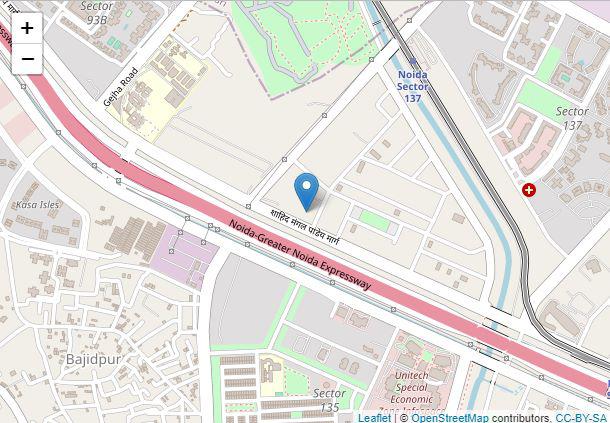
widget1 <- leaflet() %>%
  addTiles() %>%
  addMarkers(lng = 77.39902539926143, lat = 28.505037217956442,
             popup = "GeeksForGeeks Office")

# Create a simple networkD3 widget
src <- c("A", "A", "A", "A",
        "B", "B", "C", "C","K","K")
target <- c("B", "C", "D", "J",
            "E", "F", "G", "H","G","H")
networkData <- data.frame(src, target)

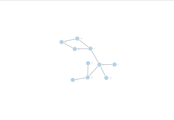
widget2 <- simpleNetwork(networkData)

# Create a simple DT widget
widget3 <- datatable(mtcars)

```

<!-- now lets view the widgets -->
```{r}
widget1
widget2
widget3
```

Output:

Widget2:

Widget3:

For the above code ensure that the libraries leaflet, networkD3 and DT are installed beforehand in your system. To install any library use the following command in the R console.

Widget 1

We have used the leaflet library for interactive maps and marked a specific location in the map as an example. Each part of the code is explained below.

• '%>% ‘ is the pipe operator which is used to chain multiple function calls together by taking output from the previous function call and passing it as the first argument to the next function call. It allows for a more concise and readable code structure.
• addTiles() function adds the default tile layer to the leaflet widget which forms the base layer of the map.
• addMarkers()the function adds markers to the leaflet widget. It takes parameters such as lng (longitude), lat (latitude), and popup (text displayed when clicking on the marker).

Widget 2

We have used the networkD3 library to create D3 JavaScript network graphs from R. Each part of the code has been explained below.

• The src and target variables are simple arrays in R. The c() function is short for “combine” or “concatenate” and is used to concatenate elements into a vector.
• networkData <- data.frame(src, target) creates a data frame called networkData by combining the src and target vectors. Each row in the data frame represents a link in the network, where the src column corresponds to the source node and the target column corresponds to the target node.
• widget2 <- simpleNetwork(networkData) creates the networkD3 widget called widget2 using the simpleNetwork function. The networkData data frame is passed as an argument to the function.

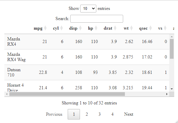
Widget 3

We have used the DT library which helps in creating interactive tables in HTML.

• The datatable function takes the mtcars dataset as input, which is a built-in dataset in R containing information about various car models. The function converts the mtcars dataset into an interactive HTML table.