How To Create A Pictograph In Excel?

The Pictograph is the record consisting of pictorial symbols. Generally, in mathematics, it is represented by the help of graphs with pictures or icons representing certain quantities or numbers of people, books, etc. It is also known as pictogram, pictogramme, pictorial chart, picture graph, or simply picto. Usually, it is used to represent the statistical data and makes it easier to understand and analyze using pictographs.

Advantages of using pictograph

It is proven that psychologically, human being finds it easier to read and interpret pictures and images. Following are the example of using a pictograph.

1. It helps kids and children to associate with numbers and objects very easily.
2. A Pictograph makes the statistical data very interesting and easy to visualize and understand.
3. It also helps in visually formatting the statistics.
4. It is also very useful to represent a very large amount of data.

In this example, we will use excel to represent the number of employees on the basis of their age group using pictographs.

Step By Step Implementation to Create A Pictograph In Excel

Step 1: Create A Dataset

In this step, we will create a dataset for our graph. We will use two columns with the titles “Age Group” and “Number Of Employees” and insert some random data.

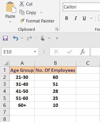
Fig 2 – Dataset

Step 2: Insert Chart

In this step, we will create our chart using the above dataset. In order to insert a chart, we need to select out data and then go to,

Insert > Charts > Insert Bar Chart. 

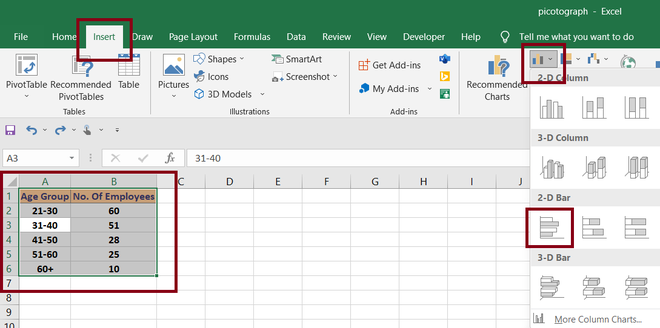
Fig 3 – Insert Bar Chart

After the above operation, excel will automatically insert the chart depending on the dataset. Below is the screenshot attached for our chart.

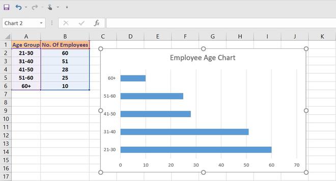
Fig 4 – Chart

Step 3: Format Data Series

In this step, we will format our data series. i.e., the data bars. For this, 

Select Bar > Right-Click > Format Data Series. 

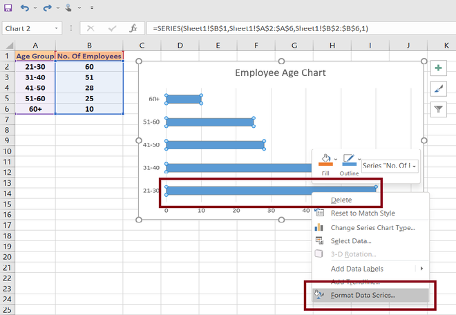
Fig 5 – Format Data Series

Once we click on Format Data Series, this will open a format data series side pane in excel where we can format our data bars according to our use.

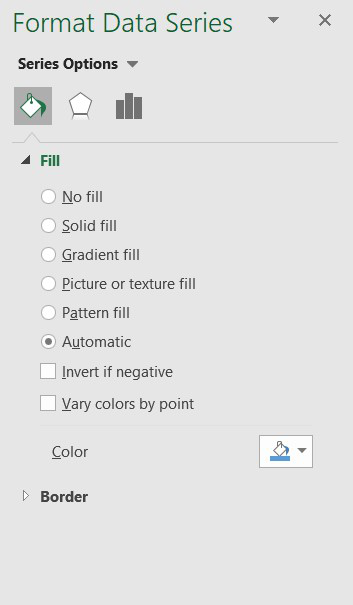
Fig 6 – Format Data Series

Step 4: Insert Picture In Data Bars

In this step, we will insert pictures in our data bars of the graph. For this, we need to go to, 

Fill > Picture or texture fill.

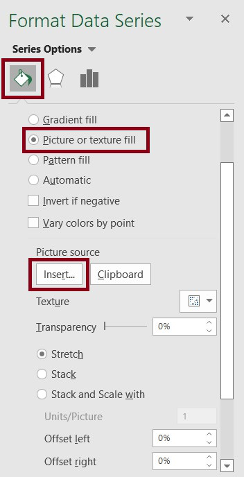
Fig 7 – Insert Picture

Once we click on the Insert button, the excel will ask us to insert an icon(Here, we are using default icons provided by excel. You can use your own icons or picture).

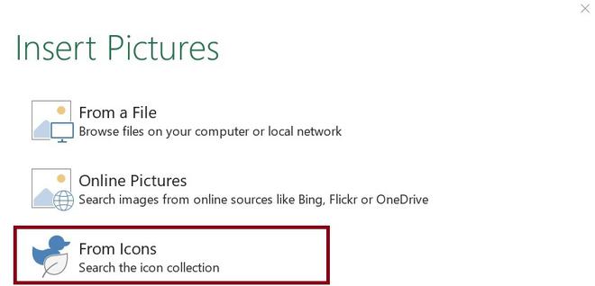
Fig 8 – Insert Default Icons

Here, we are using Employee icons to fill in the data bars.

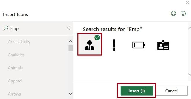
Fig 9 – Employee Icon

Once we Insert the employee icon from the default icons provided by excel, we need to use some validations regarding the inserted picture or icons.

Fig 10 – Stack Validation

1. Stretch: This will stretch one single image incomplete data bar.
2. Stack: This will represent the stacked images in the data bar.
3. Stack and Scale with: This will show the images depending on the data count.

Step 5: Output

In this step, we will see the complete pictograph of our dataset.

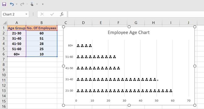
Fig 11 – Pictograph