Feature Transformations with Ensembles of Trees in Scikit Learn

An ensemble of trees is an efficient technique that can be used to combine multiple weak learners into a strong learner. The main idea of the ensemble for trees is that we take aggregate of the results from multiple trees which may not have been able to perform well. This aggregate mitigates the weaknesses of individual trees and therefore improves the performance. Scikit Learn provides multiple algorithms to determine the importance of each feature and thereby apply feature transformation.

Scikit Learn is a popular Machine Learning library that can be used for implementing feature engineering, and various machine learning algorithms. It also provides a comprehensive set of tools for working with ensembles of trees. In this article, we will discuss two main ensemble techniques based on trees.

What is an Ensemble of Trees?

Let’s say you are training a model on a huge dataset, you cleaned the data, used all the appropriate techniques of feature engineering, and selected the best features. Now, you train the model by hyper tuning and have set the most optimal set of parameters. However, you still see that your model doesn’t meet your requirements for accuracy. At this point, even if everything is in place you don’t get the most accurate results. You can say that this model is a weak learner.

Since you stubbornly want to have a model with high accuracy you need to do something that will turn this weak learner into the strong learner. This is where the ensemble of trees comes into the scene. The word ensemble here actually means “a group of things taken as a whole”. In the ensemble trees, we have multiple decision trees, each receiving the same input and producing an output. Finally, the aggregate of the output of all the trees is taken to make our model a strong learner.

In general, there are two types of ensemble techniques, i.e bagging and boosting.

• Bagging – It works by providing subsets of training data to different models and then taking majority vote(in case of classification) or average(in case of regression).
• Boosting– It works by connecting the weak learners sequentially such that output of one model is sent as input to next model for improvement.

In both the cases, we get a model that has improved high accuracy.

How ensemble models work?

Both ensemble models work by combing the predictions of multiple trees, however there are slight differences. In case of Gradient Boosting Classifier each tree is built iteratively or sequentially based on the aggregate performance of the trees build so far. Whereas, in Random Forest Classifier, the tree is built independently and then the result of all trees is aggregated to produce an output.

We know that in each case a decision tree is built. A decision tree and multiple nodes and leaf nodes. When you input any data x and it goes through the tree then it ends up in one of the leaf node. If you have trained the model with N decision trees, each decision tree will have multiple leaf nodes as show below:

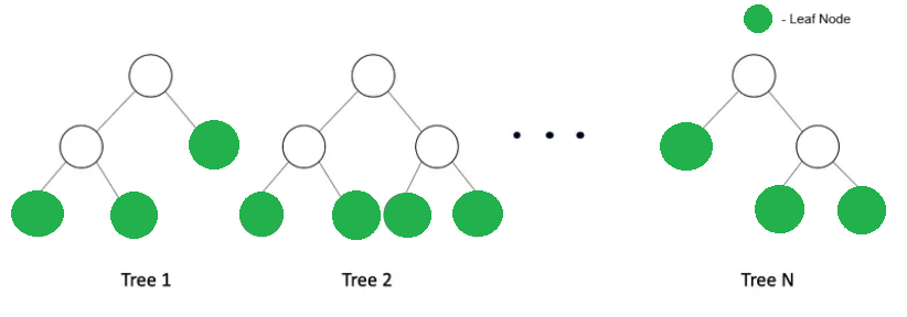
As we know, from each of these trees only one leaf node will get activated. If we use one hot encoder, then for each tree we will get a vector.In this vector, the value will be 1 for the leaf node which is activated and 0 for the rest of the leaf nodes. Hence, for N number of trees in a trained model you will have N one hot encoded vectors. When we concatenate all these one hot encode vector what we get it is a transformed feature vector. Thus, this transformation actually makes the dense vector into sparse vector.

Random Forest Classifier

The working of random forest classifier is quite simple. In a normal decision tree algorithm, you have one single decision tree through which you pass the input and get the output as result. When working with random forest classifier, you have multiple such decision trees. Each decision tree gets different subset of data points and different subset of features randomly. Now, when this input data is passed to different decisions tree, we get an output from each tree.

The majority vote is taken if you are dealing with classification problem. For regression problems, you take average of the outputs received. Since each tree has seen almost different data points and features it would be more accurate when aggregated and will not overfit. Here, the model truly understands the underlying pattern.

Let’s use Random Forest Classifier for feature transformation.

Importing Libraries and Splitting Data

Firstly, we create a random dataset using the make_classification method and then split it into train and test data.

Python

from sklearn.datasets import make_classification
from sklearn.model_selection import train_test_split

# Create a synthetic dataset for illustration
X, y = make_classification(n_samples=1000, n_features=20, random_state=42)
X_train, X_test, y_train, y_test = train_test_split(X, y, test_size=0.2, random_state=42)

Implementing Random Forest Classifier

Python3

from sklearn.ensemble import RandomForestClassifier

# Train a Random Forest classifier
rf_classifier = RandomForestClassifier(n_estimators=100, random_state=42)
rf_classifier.fit(X_train, y_train)

When we create a random forest classifier model we will pass n_estimators=100, which means the number of trees in forest is set to 100. random_state will control the randomness of bootstrapping of samples used while building trees and sampling of features.

Feature Importance

Python3

# Get feature importances
feature_importances = rf_classifier.feature_importances_

# Use feature importances for feature selection or transformation
selected_features_X_train = X_train[:, feature_importances > 0.02]
selected_features_X_test = X_test[:, feature_importances > 0.02]

print(feature_importances)

Output:

[0.01695078 0.10181962 0.02108998 0.01368187 0.01554572 0.36313417
 0.02333904 0.01519547 0.01549653 0.0158737  0.01915803 0.02569037
 0.01922067 0.01651946 0.07557534 0.01734487 0.01852994 0.01427792
 0.17725206 0.01430447]

We can use the feature_importances_ property of RandomForestClassifier to know which features are important. In our case, we select only the features which have feature_importances_ value greater than 0.02. This actually trims down our columns from 20 to 7, i.e. only 7 significant features are selected to classify.

When you print the feature_importances you will get a list that contains the importance of each feature in classification. The importance of a feature is calculated based on how much that feature contributes to reducing impurity in decision tree.

Logistic Regression

You can train the Logistic Regression model directly with the splitted dataset and also with the dataset on which we performed feature transformation just now.

Python3

from sklearn.linear_model import LogisticRegression

model1 = LogisticRegression()
model1.fit(X_train, y_train)

model2 = LogisticRegression()
model2.fit(selected_features_X_train, y_train)

This code trains two models using the Logistic Regression module of scikit-learn. While the second model (model2) is trained on a subset of features (selected_features_X_train and y_train), the first model (model1) is trained on the entire feature set (X_train and y_train). The utilization of specific features in the second model indicates a desire to enhance the model’s performance by concentrating on particular predictors and maybe going through a feature selection or dimensionality reduction procedure.

Evaluation

Python3

score1 = model1.score(X_test, y_test)
score2 = model2.score(selected_features_X_test, y_test)

print("Mean accuracy without ensemble of tree: ", score1)
print("Mean accuracy with ensemble of tree: ", score2)

Output:

Mean accuracy without ensemble of tree:  0.855
Mean accuracy with ensemble of tree:  0.875

When you compare the mean accuracy score you can see that it has been significantly improved by 0.02 after performing feature transformation.

Since this was a custom dataset created by us you may not notice a huge change or difference in accuracy. However, depending on the use cases and real datasets you can expect Random Forest to be a helpful technique.

Gradient Boosting Classifier

In gradient boosting classifier, each model tries to reduce the errors of the preceding model. All such models are arranged in sequentially so that we get a final output having high accuracy. It is important to note that rather than fitting the model again, it tries to fit a new model to the residual errors made by the previous one. Thus, it boosts the performance overall.

To get started you need to import the following form sklearn.

Importing Libraries

Python3

from sklearn.ensemble import GradientBoostingClassifier
from sklearn.datasets import make_classification
from sklearn.model_selection import train_test_split
from sklearn.linear_model import LogisticRegression

Generating Data and splitting data

Python3

# Create a synthetic dataset for illustration
X, y = make_classification(n_samples=1000, n_features=20, random_state=42)
X_train, X_test, y_train, y_test = train_test_split(X, y, test_size=0.2, random_state=42)

We will be generating synthetic dataset using make_classification() and then split it into training and testing dataset.

Training a Gradient Tree classifier

Python3

# Train a Gradient Boosted Trees classifier
gb_classifier = GradientBoostingClassifier(n_estimators=100, random_state=42)
gb_classifier.fit(X_train, y_train)

When you create a GradientBoostingClassifier model you need to specify n_estimators which means the number of boosting stages to perform. By default, n_estimators is set to 100.

Feature importance

Python3

# Get feature importances
feature_importances = gb_classifier.feature_importances_

# Use feature importances for feature selection or transformation
selected_features_X_train = X_train[:, feature_importances > 0.02]
selected_features_X_test = X_test[:, feature_importances > 0.02]

print(feature_importances)

Output:

[0.00528748 0.01243391 0.01087386 0.00099458 0.00248339 0.66505179
 0.01199457 0.01062141 0.00485092 0.00563588 0.00230154 0.01865276
 0.01184804 0.00581178 0.17462893 0.00929922 0.00624585 0.00471869
 0.03393672 0.00232869]

You can know the importance of each feature by calling the feature_importances_ property. It gives you a list containing importance value for each feature. Then we select only those features which have feature_importances_ greater than 0.02

If you print feature_importances, you will get an array of values where each value corresponds to the importance of a specific feature. Higher value means more importance.

Training the model

Python3

#Logistic Regression without Gradient Boosting Classifier
model1 = LogisticRegression()
model1.fit(X_train, y_train)

#Logistic Regression with Gradient Boosting Classifier
model2 = LogisticRegression()
model2.fit(selected_features_X_train, y_train)

Now, we train two models. One with GradientBoostingClassifier and another without it.

Evaluation

Python3

score1 = model1.score(X_test, y_test)
score2 = model2.score(selected_features_X_test, y_test)

print("Mean accuracy without ensemble of tree: ", score1)
print("Mean accuracy with ensemble of tree: ", score2)

Output:

Mean accuracy without ensemble of tree:  0.855
Mean accuracy with ensemble of tree:  0.865

When we compare the two models based on their mean accuracy we see that the accuracy improves when we apply feature transformation by using GradientBoostingClassifier.

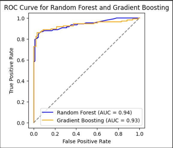
ROC Curve

Since, we have learned to use both the techniques of ensemble, we will compare them using ROC curve

Python3

from sklearn.metrics import roc_curve, roc_auc_score
import matplotlib.pyplot as plt

# Predict probabilities for positive class
y_probs_rf = rf_classifier.predict_proba(X_test)[:, 1]
y_probs_gb = gb_classifier.predict_proba(X_test)[:, 1]

# Calculate ROC curve
fpr_rf, tpr_rf, _ = roc_curve(y_test, y_probs_rf)
fpr_gb, tpr_gb, _ = roc_curve(y_test, y_probs_gb)

# Calculate AUC (Area Under the Curve) score
auc_rf = roc_auc_score(y_test, y_probs_rf)
auc_gb = roc_auc_score(y_test, y_probs_gb)

# Plot ROC curve
plt.figure(figsize=(4, 4))
plt.plot(fpr_rf, tpr_rf, color='blue', label=f'Random Forest (AUC = {auc_rf:.2f})')
plt.plot(fpr_gb, tpr_gb, color='orange', label=f'Gradient Boosting (AUC = {auc_gb:.2f})')
plt.plot([0, 1], [0, 1], color='gray', linestyle='--')  # Diagonal line for reference
plt.xlabel('False Positive Rate')
plt.ylabel('True Positive Rate')
plt.title('ROC Curve for Random Forest and Gradient Boosting')
plt.legend()
plt.show()

Output:

ROC Curve

For two classifiers, Random Forest (rf_classifier) and Gradient Boosting (gb_classifier), this code snippet assesses the Receiver Operating Characteristic (ROC) curves and Area Under the Curve (AUC) scores. By utilizing both classifiers, it initially forecasts the test set’s positive class probabilities. The ROC curves of each classifier are then used to compute the False Positive Rate (fpr) and True Positive Rate (tpr). The classifiers’ discrimination performance is measured by computing the AUC scores. Lastly, a diagonal reference line and the ROC curves for each classifier are plotted by the code, along with the corresponding AUC scores.

Conclusion

To sum up, using ensembles of trees and feature transformations in Scikit-Learn provides a strong way to improve predictive modeling. The combined strength of several decision trees is tapped into by methods like Random Forests and Gradient Boosting, which make it possible to handle complex relationships in the data effectively. The automatic selection of relevant predictors is aided by the natural identification of feature importance through ensemble methods. This increases the accuracy of the model and offers insightful information about the importance of various features. Through the integration of feature transformations and tree-based ensembles, Scikit-Learn provides a stable framework to handle complex patterns in a variety of datasets, thereby advancing machine learning solutions that are more comprehensible and efficient.