Feature agglomeration in Scikit Learn

Data Science is a wide field with a lot of hurdles that data scientist usually faces to get informative insights out of the data presented to them, one of such hurdles is referred to as ‘The Curse of Dimensionality’. As the number of data features increases in the dataset the complexity of modelling the dataset increases exponentially, and capturing meaningful patterns in the data becomes more difficult. In this article, we will dive deep into the Feature Agglomeration process which is a feature reduction method and helps in realizing data in a better way.

Feature Agglomeration

In machine learning, dimensionality reduction is achieved through feature agglomeration. By combining related features, it seeks to extract pertinent details while lowering the dataset’s total dimensionality. It improves computing efficiency and interpretability by grouping related features into clusters. Fewer composite features are produced as a result of the algorithm’s hierarchical merging of pairwise associations between features. The most illuminating elements of the original data are preserved during this procedure, which helps with tasks like grouping and classification. By concentrating on pertinent feature groups, feature agglomeration can be especially helpful when working with high-dimensional datasets, increasing productivity and possibly even enhancing model performance.

Working of Feature Agglomeration

The main goal of feature agglomeration is to group similar correlated features and make clusters out of them, here we will be discussing how the feature agglomeration works behind the curtain:

• Each feature is considered as a separate cluster initially, if ‘n’ number of features are present then ‘n’ clusters will be formed.
• After the above step distance between each feature clusters are measured by the affinity parameter which we mention while initializing the feature agglomeration.
• In this step the grouping of the clusters happen, the closest clusters according to the distance are merged together into a single cluster and this step is repeated until only ‘n_clusters’ amount of clusters are left.
• After each merge the pairwise distances are updated with the new clusters formed and the existing clusters.
• The steps are repeated until the required number of clusters are achieved.
• Once the stage of remaining ‘n_clusters’ is reached each cluster gets represented by a feature. The value of ‘pooling’ parameter determines the way in which the new features are going to be represented, for example if we set the value of pooling parameter of be ‘mean’ it will represent the mean value.
• At last the original features are transformed by replacing the existing features with the new features that are formed by feature agglomeration.

Parameters That Shape The Clustering

Here we will be discussing some of the most important parameters of feature agglomeration which can help us understand the topic thoroughly and help us in generating better combination of features.

• n_clusters: This parameter defines the number of clusters that must form after feature agglomeration is done, the value of ‘n_clusters’ tells us about the final features that will be used in our model training and testing. It helps eliminating the extra features that are not useful in model performance and combines them to the closest cluster. ‘n_clusters’ can have any numeric value but we must be careful in choosing this parameter’s value since it might also deteriorate our model performance if not chosen correctly.
• affinity: This parameter defines how the distance between the clusters is going to be recorded, by changing the value of this ‘affinity’ parameter the change in structure of the clusters might be observed. It can have different values including “l1”, “l2”, “Manhattan“, “Euclidean” etc.
• linkage: This parameter species the method used to calculate distance between clusters during feature agglomeration process. It can have different values including “ward” – this value minimizes the variance between the clusters, “complete” – this value calculates the maximum value between all data points in two clusters, “average” – this value calculates the average value of distances between two clusters, “single” – this method calculates the minimum value between data points between two clusters.
• pooling_func: This parameter combines the values of agglomerated features into a final cluster feature, in feature agglomeration the features of a dataset gets reduced in a certain way when correlated similar features are getting bundled together the different values of those features are getting arranged according to the ‘pooling_func’ parameter. It can have different values such as ‘mean’, ‘median’ etc. This parameter takes different correlated features and combines them and returns an array of combined values.

Implementation of Feature Agglomeration

Now we will be applying Feature Agglomeration on Iris dataset to reduce the total features, this dataset consists of four features namely Sepal Length in cm, Sepal Width in cm, Petal Length in cm, Petal Width in cm and from these features we have to reduce the total features equal to the mentioned ‘n_clusters’ value. We will be applying feature agglomeration through ‘sklearn’ and reduce the total number of feature from four to two. The iris flower dataset could be obtained from here.

Importing Libraries

Python3

import pandas as pd
from sklearn.cluster import FeatureAgglomeration
from sklearn.preprocessing import StandardScaler
from sklearn.pipeline import make_pipeline

This code uses scikit-learn to illustrate feature aggregation. Pandas is used to load the Iris dataset, after which features are separated and the data is standardized. A pipeline is then used to apply feature agglomeration using two clusters. When comparing the original and changed datasets, a scatter plot is made to show how feature aggregation affects the first two features. The transformed data is then printed.

Loading Dataset

Python3

# Loading the iris dataset
data = pd.read_csv("Iris.csv", index_col=0)

Using the first column as the index, this code reads the Iris dataset from a CSV file (“Iris.csv”) into a pandas Data Frame.

Mapping labels and separating features

Python3

# Mapping string labels to numerical values
species_mapping = {'Iris-setosa': 0, 'Iris-versicolor': 1, 'Iris-virginica': 2}
data['Species'] = data['Species'].map(species_mapping)


# Separating features
X = data.drop("Species", axis=1)

To translate Iris species’ string labels into numerical values, this function builds a mapping dictionary (species_mapping). Next, it uses this mapping to the dataset’s “Species” column, substituting the relevant numerical values (0 for “Iris-setosa,” 1 for “Iris-versicolor,” and 2 for “Iris-virginica”) for the string labels. Lastly, the result is assigned to variable X and the features are separated by removing the ‘Species’ column from the Data Frame.

Standard scaling

Python3

# Standardizing the dataset
scaler = StandardScaler()
# This line transforms the dataset and stores the new dataset
X_scaled = scaler.fit_transform(X)

The dataset will be standardized by using a StandardScaler object (scaler) from scikit-learn, which is initialized using this code. Next, the feature matrix X is transformed with the fit_transform method to have a zero mean and a unit variance. X_scaled is the variable that contains the standardized dataset. Making sure that all characteristics have similar sizes is essential for many machine learning algorithms, and this procedure makes that happen.

Implementing Feature Agglomeration

Python3

n_clusters = 2  # Number of clusters (desired number of output features)

# Creating a FeatureAgglomeration model with n_clusters equals 2
agglomeration = FeatureAgglomeration(n_clusters=n_clusters)

The desired number of clusters, or output characteristics, is indicated by setting the variable n_clusters to 2 by this code. After that, it builds a FeatureAgglomeration model from scikit-learn called agglomeration with the desired number of clusters. Feature agglomeration is a dimensionality reduction strategy that preserves significant information in the data while lowering the total number of features by grouping related features together.

Creating a pipeline and fitting the data

Python3

# Creating a pipeline with scaling and feature agglomeration
pipeline = make_pipeline(scaler, agglomeration)

# Fitting and transforming the data
X_transformed = pipeline.fit_transform(X)

This code uses scikit-learn to develop a machine learning pipeline. The previously described scaler and agglomeration phases are combined into a single pipeline called pipeline using the make_pipeline function. This process is then used to fit and transform the dataset X, producing the transformed dataset X_transformed. Pipelines are helpful for efficiently planning, arranging, and carrying out a series of modeling and data processing operations.

Comparing the original and transformed data

Python3

# Comparing the shapes of original vs transformed data
print("Original shape:", X.shape)
print("Transformed shape:", X_transformed.shape)

# printing the first rows of the transformed dataset
print("\nHere's the first five rows of transformed Dataframe:\n")
print(X_transformed[:5, :])

Output:

Original shape: (150, 4)
Transformed shape: (150, 2)
Here's the first five rows of transformed Dataframe:
[[-1.18497677  1.03205722]
 [-1.26575535 -0.1249576 ]
 [-1.36548916  0.33784833]
 [-1.36796798  0.10644536]
 [-1.22536606  1.26346019]]

The forms of the original dataset X and the converted dataset X_transformed are compared and shown in the first print statement. The converted dataset’s first five rows are shown in the second print statement, giving readers an idea of how the data has been modified following feature aggregation. This facilitates comprehension of the feature aggregation process’s effects on the dataset.

Plotting original data

Python3

# Plotting the original data
plt.figure(figsize=(10,5 ))
# Plotting the first two columns of the original data
plt.subplot(1, 2, 2)
plt.scatter(X.iloc[:, 0], X.iloc[:, 1], c=data['Species'], cmap='viridis')
plt.title('Original Data (First Two Features)')
plt.xlabel('Original Feature 1')
plt.ylabel('Original Feature 2')

plt.tight_layout()
plt.show()

Output:

The first two columns of the original data are shown as a scatter plot in the subplot on the right. Using the ‘viridis’ colormap, the dots are colored according to the species labels found in the ‘Species’ column. The narrative sheds light on how the original features were distributed and related to one another.

Plotting the transformed data

Python3

# Plotting the transformed data
plt.figure(figsize=(10, 5))

# Plotting the first two columns of the transformed data
plt.subplot(1, 2, 1)
plt.scatter(X_transformed[:, 0], X_transformed[:, 1],
            c=data['Species'], cmap='viridis')
plt.title('Transformed Data (First Two Features)')
plt.xlabel('Transformed Feature 1')
plt.ylabel('Transformed Feature 2')
plt.tight_layout()
plt.show()

Output:

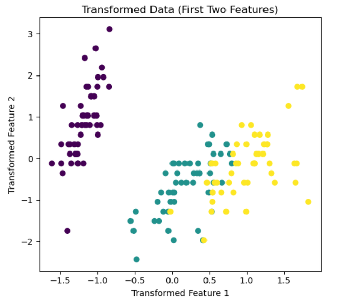
The modified dataset is visualized via this code. A scatter plot of the first two columns of the modified data can be seen in the subplot on the left. Using the ‘viridis’ colormap, the dots are colored according to the species labels in the ‘Species’ column. This graphic shows how the distribution and associations of the altered features have changed as a result of feature agglomeration. Plots are displayed using plt.show(), and appropriate spacing between subplots is guaranteed using plt.tight_layout().

Advantages and Disadvantages of Feature Agglomeration

Advantages

• As a main objective of feature agglomeration, it helps reducing the number of extra features in the dataset grouping similar features together and therefore reducing the complexity of data exploration.
• Grouping of similar function may reduce the noise in the data and help in understanding better relationship in data.
• Reduction of extra features may also improve the model performance.

Disadvantages

• Feature agglomeration may reduce the descriptive information of the data present originally.
• If the parameters of feature agglomeration not chosen wisely may result into loss of informative details about the data.
• In some cases feature agglomeration might not provide significant benefits as compared to the original data which was present previously.