Feature Subset Selection Process

Feature Selection is the most critical pre-processing activity in any machine learning process. It intends to select a subset of attributes or features that makes the most meaningful contribution to a machine learning activity. In order to understand it, let us consider a small example i.e. Predict the weight of students based on the past information about similar students, which is captured inside a ‘Student Weight’ data set. The data set has 04 features like Roll Number, Age, Height & Weight. Roll Number has no effect on the weight of the students, so we eliminate this feature. So now the new data set will be having only 03 features. This subset of the data set is expected to give better results than the full set. 

Age	Height	Weight
12	1.1	23
11	1.05	21.6
13	1.2	24.7
11	1.07	21.3
14	1.24	25.2
12	1.12	23.4

The above data set is a reduced dataset. Before proceeding further, we should look at the fact why we have reduced the dimensionality of the above dataset OR what are the issues in High Dimensional Data?

High Dimensional refers to the high number of variables or attributes or features present in certain data sets, more so in the domains like DNA analysis, geographic information system (GIS), etc.  It may have sometimes hundreds or thousands of dimensions which is not good from the machine learning aspect because it may be a big challenge for any ML algorithm to handle that. On the other hand, a high quantity of computational and a high amount of time will be required. Also, a model built on an extremely high number of features may be very difficult to understand. For these reasons, it is necessary to take a subset of the features instead of the full set. So we can deduce that the objectives of feature selection are:

1. Having a faster and more cost-effective (less need for computational resources) learning model
2. Having a better understanding of the underlying model that generates the data.
3. Improving the efficacy of the learning model.

Main Factors Affecting Feature Selection

a. Feature Relevance: In the case of supervised learning, the input data set (which is the training data set), has a class label attached. A model is inducted based on the training data set — so that the inducted model can assign class labels to new, unlabeled data. Each of the predictor variables, ie expected to contribute information to decide the value of the class label. In case of a variable is not contributing any information, it is said to be irrelevant. In case the information contribution for prediction is very little, the variable is said to be weakly relevant. The remaining variables, which make a significant contribution to the prediction task are said to be strongly relevant variables.

In the case of unsupervised learning, there is no training data set or labelled data. Grouping of similar data instances are done and the similarity of data instances are evaluated based on the value of different variables. Certain variables do not contribute any useful information for deciding the similarity of dissimilar data instances. Hence, those variable makes no significant contribution to the grouping process. These variables are marked as irrelevant variables in the context of the unsupervised machine learning task. 

We can understand the concept by taking a real-world example: At the start of the article, we took a random dataset of the student. In that, Roll Number doesn’t contribute any significant information in predicting what the Weight of a student would be. Similarly, if we are trying to group together students with similar academic capabilities, Roll No can really not contribute any information. So, in the context of grouping students with similar academic merit, the variable Roll No is quite irrelevant.  Any feature which is irrelevant in the context of a machine learning task is a candidate for rejection when we are selecting a subset of features.

b. Feature Redundancy: A feature may contribute to information that is similar to the information contributed by one or more features. For example, in the Student Data-set, both the features Age & Height contribute similar information. This is because, with an increase in age, weight is expected to increase. Similarly, with the increase in Height also weight is expected to increase. So, in context to that problem, Age and Height contribute similar information. In other words, irrespective of whether the feature Height is present or not, the learning model will give the same results. In this kind of situation where one feature is similar to another feature, the feature is said to be potentially redundant in the context of a machine learning problem. 

All features having potential redundancy are candidates for rejection in the final feature subset. Only a few representative features out of a set of potentially redundant features are considered for being a part of the final feature subset. So in short, the main objective of feature selection is to remove all features which are irrelevant and take a representative subset of the features which are potentially redundant. This leads to a meaningful feature subset in the context of a specific learning task. 

The measure of feature relevance and redundancy

a. Measures of Feature Relevance: In the case of supervised learning, mutual information is considered as a good measure of information contribution of a feature to decide the value of the class label. That is why it is a good indicator of the relevance of a feature with respect to the class variable. The higher the value of mutual information of a feature, the more relevant is that feature. Mutual information can be calculated as follows:

Where, marginal entropy of the class, (

Marginal entropy of the feature ‘x’, 

And K = number of classes, C = class variable, f = feature set that take discrete values. In the case of unsupervised learning, there is no class variable. Hence, feature-to-class mutual information cannot be used to measure the information contribution of the features. In the case of unsupervised learning, the entropy of the set of features without one feature at a time is calculated for all features. Then the features are ranked in descending order of information gain from a feature and the top percentage (value of beta is a design parameter of the algorithm) of features are selected as relevant features. The entropy of a feature f is calculated using Shannon’s formula below:

 is used only for features that take the discrete values. For continuous features, it should be replaced by discretization performed first to estimate the probabilities p(f=x).

b. Measures of Feature Redundancy: There are multiple measures of similarity of information contribution, the main ones are:

• Correlation-based Measures
• Distance-based Measures
• Other coefficient-based Measure

1. Correlation Based Similarity Measure

Correlation is a measure of linear dependency between two random variables. Pearson’s product correlation coefficient is one of the most popular and accepted measures correlation between two random variables. For two random feature variables F₁ and F₂ , the Pearson coefficient is defined as:

 where 

  where 

Correlation value ranges between +1 and -1. A correlation of 1 (+/-) indicates perfect correlation. In case the correlation is zero, then the features seem to have no linear relationship. Generally for all feature selection problems, a threshold value is adopted to decide whether two features have adequate similarity or not.

2. Distance-Based Similarity Measure

The most common distance measure is the Euclidean distance, which, between two features F₁ and F₂ are calculated as:

Where the features represent an n-dimensional dataset. Let us consider that the dataset has two features, Subjects (F₁) and marks (F₂) under consideration. The Euclidean distance between the two features will be calculated like this:

Subjects (F1)	Marks (F2)	(F1 -F2)	(F1 -F2)2
2	6	-4	16
3	5.5	-2.5	6.25
6	4	2	4
7	2.5	4.5	20.25
8	3	5	25
6	5.5	0.5	0.25
6	7	-1	1
7	6	1	1
8	6	2	4
9	7	2	4

A more generalized form of the Euclidean distance is the Minkowski Distance, measured as 

Minkowski distance takes the form of Euclidean distance (also called L₂ norm) where r = 2. At r=1, it takes the form of Manhattan distance (also called L₁ norm) : 

3. Other Similarity Measures

Jaccard index/coefficient is used as a measure of dissimilarity between two features is complementary of Jaccard Index. For two features having binary values, Jaccard Index is measured as: 

Where   = number of cases when both the feature have value 1,

=  number of cases where the feature 1 has value 0 and feature 2 has value 1,

=  the number of cases where feature 1 has value 1 and feature 2 has value 0.

Jaccard distance: 

Let us take an example to understand it better. Consider two features, F₁ and F₂ having values (0, 1, 1, 0, 1, 0, 1, 0) and (1, 1, 0, 0, 1, 0, 0, 0). 

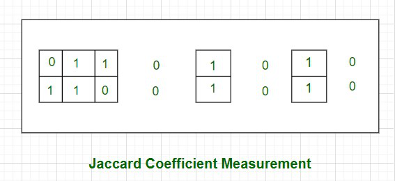
As shown in the above picture, the cases where both the values are 0 have been left out without border- as an indication of the fact that they will be excluded in the calculation of the Jaccard coefficient. 

Jaccard coefficient of F₁ and F₂ , J = 

Therefore, Jaccard Distance between those two features is d_j = (1 – 0.4) = 0.6

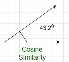
Note: One more measure of similarity using similarity coefficient calculation is Cosine Similarity. For the sake of understanding, let u stake an example of the text classification problem. The text needs to be first transformed into features with a word token being a feature and the number of times the word occurs in a document comes as a value in each row. There are thousands of features in such a text dataset. However, the data set is sparse in nature as only a few words do appear in a document and hence in a row of the data set. So each row has very few non-zero values. However, the non-zero values can be anything integer value as the same word may occur any number of times. Also, considering the sparsity of the dataset, the 0-0 matches need to be ignored. Cosine similarity which is one of the most popular measures in text classification is calculated as:

Where, x.y is the vector dot product of x and y  = 

  and 

So let’s calculate the cosine similarity of x and y, where x = (2,4,0,0,2,1,3,0,0) and y = (2,1,0,0,3,2,1,0,1). In this case, dot product of x and y will be x.y = 2*2 + 4*1 + 0*0 + 0*0 + 2*3 + 1*2 + 3*1 + 0*0 + 0*1 = 19.

Cosine Similarity measures the angle between x and y vectors. Hence, if cosine similarity has a value of 1, the angles between x and y is 0 degrees which means x and y are the same except for the magnitude. If the cosine similarity is 0, the angle between x and y is 90⁰. Hence, they do not share any similarity. In the case of the above example, the angle comes out to be 43.2⁰. 

Even after all these steps, there are some few more steps. You can understand it by the following flowchart:

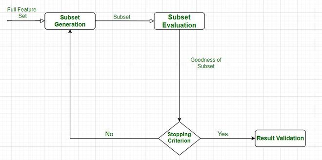
Feature Selection Process

After the successful completion of this cycle, we get the desired features, and we have finally tested them also.

The feature subset selection process involves identifying and selecting a subset of relevant features from a given dataset. It aims to improve model performance, reduce overfitting, and enhance interpretability. Here is a general outline of the feature subset selection process:

Data Preparation:

Clean the data: Handle missing values, outliers, and data inconsistencies.
Encode categorical variables: Convert categorical features into numerical representations, such as one-hot encoding or label encoding.
Normalize or standardize numerical features: Scale numerical features to a common range to avoid bias.

Feature Ranking/Scoring:

Select an appropriate feature scoring or ranking method based on the nature of the data and the problem you are addressing. Common scoring methods include correlation coefficient, information gain, chi-square test, mutual information, or statistical tests like t-test or ANOVA.
Calculate the score or rank for each feature based on its relationship with the target variable.

Feature Selection Techniques:

Filter-based methods: Select features based on their individual scores or rankings. Set a threshold and select features above that threshold.
Wrapper-based methods: Use a machine learning model with different feature subsets and evaluate their performance to determine the optimal subset. Techniques like forward selection, backward elimination, or recursive feature elimination fall under this category.
Embedded methods: Incorporate feature selection as part of the model training process. Algorithms like Lasso (L1 regularization) and Ridge (L2 regularization) can automatically select relevant features during model training.

Evaluate Subset Performance:

Split the dataset into training and validation sets.
Train a machine learning model using the selected subset of features.
Evaluate the model’s performance metrics (e.g., accuracy, precision, recall, F1-score, or area under the ROC curve) on the validation set.
If the performance is not satisfactory, go back to the feature selection step and try different techniques or adjust the parameters

.
Iterative Refinement:

Iterate through steps 2-4, trying different feature scoring methods, selection techniques, thresholds, or algorithms to find the optimal feature subset.
Utilize cross-validation techniques, such as k-fold cross-validation, to obtain more robust estimates of model performance and feature relevance.
Final Model Training and Testing:

Once the optimal feature subset is selected, train the final machine learning model on the entire training dataset using the selected features.
Evaluate the model’s performance on an independent test dataset to assess its generalization ability.

Interpretability and Validation:

Analyze the selected features and their relationship with the target variable to gain insights into the problem domain.
Validate the selected features on new, unseen data to ensure their robustness and effectiveness.
Remember that the feature subset selection process is iterative and may require experimenting with different techniques, thresholds, and evaluation metrics to find the most suitable subset of features for your specific problem.