Evaluating Forecast Accuracy

Evaluating forecast accuracy is a critical step in assessing the performance of time series forecasting models. It helps you understand how well your model is predicting future values compared to the actual observed values. Commonly used metrics for evaluating forecast accuracy include Mean Absolute Error (MAE), Root Mean Squared Error (RMSE), Mean Absolute Percentage Error (MAPE), and more.

Mean Absolute Error (MAE)

In R Programming Language Mean Absolute Error (MAE) measures the average absolute difference between the predicted and actual values. It provides a straightforward assessment of forecast accuracy.

Where:

• n is the number of observations.
• yi is the actual value.
• ^yi is the predicted value.

R

set.seed(123)
actual_data <- rnorm(100)
forecast_data <- actual_data + rnorm(100, sd = 0.5)

# Calculate Mean Absolute Error (MAE)
mae <- mean(abs(actual_data - forecast_data))
cat("Mean Absolute Error (MAE):", mae, "\n")

Output:

Mean Absolute Error (MAE): 0.3821047 

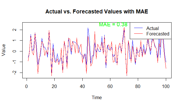
Plotting Actual vs. Forecasted Values

R

# Plotting Actual vs. Forecasted Values
plot(actual_data, type = "l", col = "blue", ylim = range(c(actual_data, forecast_data)),
     xlab = "Time", ylab = "Value", main = "Actual vs. Forecasted Values with MAE")
lines(forecast_data, col = "red")
legend("topright", legend = c("Actual", "Forecasted"), col = c("blue", "red"), lty = 1)

# Adding MAE information to the plot
text(x = 50, y = max(c(actual_data, forecast_data)),
     labels = paste("MAE =", round(mae, 2)), pos = 4, col = "green", cex = 1.2)

Output:

Root Mean Squared Error (RMSE)

Root Mean Squared Error (RMSE) is similar to MAE but gives more weight to large errors since it squares the differences before taking the average and then takes the square root.

R

# Calculate Root Mean Squared Error (RMSE)
rmse <- sqrt(mean((actual_data - forecast_data)^2))
cat("Root Mean Squared Error (RMSE):", rmse, "\n")

Output:

Root Mean Squared Error (RMSE): 0.4840658 

Scale of Measurement: The RMSE is expressed in the same units as the original data. In your case, if your original data represents some kind of measurement (e.g., temperature, sales, or any other numerical quantity), then the RMSE will be in the same units.

• Interpretation: An RMSE value of 0 indicates a perfect fit, meaning that the forecasted values exactly match the actual values. As the RMSE increases, it indicates increasing discrepancies between the predicted and actual values.
• Magnitude of Errors: The RMSE gives an average magnitude of errors. In your case, an RMSE of 0.4841 means that, on average, the difference between your predicted values and the actual values is approximately 0.4841 units.
• Comparison with Other Models: You can use the RMSE to compare the performance of different models. A lower RMSE generally indicates a better fit, but the interpretation should consider the scale of measurement and the characteristics of the data.

Mean Absolute Percentage Error (MAPE)

Mean Absolute Percentage Error (MAPE) expresses the forecast accuracy as a percentage of the absolute percentage difference between the predicted and actual values.

R

# Calculate Mean Absolute Percentage Error (MAPE)
mape <- mean(abs((actual_data - forecast_data) / actual_data)) * 100
cat("Mean Absolute Percentage Error (MAPE):", mape, "%\n")

Output:

Mean Absolute Percentage Error (MAPE): 199.7481 %

Magnitude of Percentage Errors: The MAPE is expressed as a percentage, indicating the average magnitude of the percentage errors. A MAPE of 199.7481% suggests that, on average, the absolute percentage difference between the predicted and actual values is approximately 199.7481%.

• Interpretation: MAPE is interpreted as a percentage of the actual values. For example, a MAPE of 10% would imply that, on average, the predictions deviate by 10% from the actual values.
• Comparison with Other Models: MAPE allows you to compare the accuracy of different models, and a lower MAPE generally indicates a better fit. However, like any metric, it should be interpreted considering the characteristics of the data.
• Limitations: MAPE has some limitations, such as sensitivity to zero values in the actual data. It is important to be aware of these limitations when using MAPE.

Conclusion

Evaluating forecast accuracy is crucial for understanding the performance of your time series forecasting models. By employing metrics like MAE, RMSE, and MAPE in R, you can quantify the accuracy of your predictions and make informed decisions about the effectiveness of your forecasting approach. Always adapt these metrics based on your specific needs and the characteristics of your time series data.