Early Stopping for Regularisation in Deep Learning

When training big models with enough representational capacity to overfit the task, we frequently notice that training error drops consistently over time, while validation set error rises again. 

Figure 1 shows an example of this type of behavior. This pattern is fairly consistent.

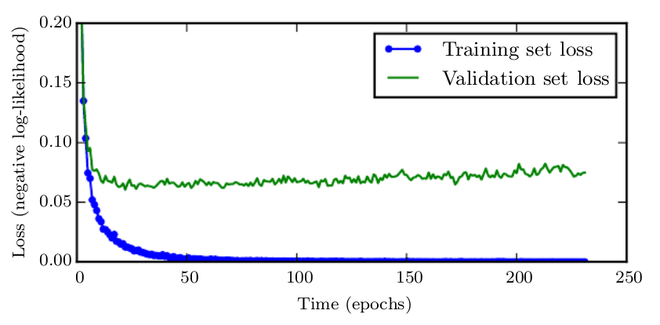
Figure 1

This means that by returning to the parameter setting at the moment in time with the lowest validation set error, we can have a model with improved validation set error (and, ideally, better test set error). We save a copy of the model parameters every time the error on the validation set improves. We return these parameters rather than the most recent parameters when the training algorithm finishes. After a predetermined number of repetitions, the algorithm stops if no parameters have improved over the best-recorded validation error. This approach is detailed in the algorithm section below. For identifying the ideal length of time to train, the algorithm shows early stopping. This meta-algorithm is a generic strategy that works with a wide range of training algorithms and error quantification methods on the validation set.

Algorithm 1:

[Tex]\text{while $j<p$ do } \\
\text{\;\;\;\;Update $\boldsymbol{\theta}$ by running the training algorithm for $n$ steps.}\\
\text{\;\;\;\;$i \leftarrow i+n$}\\
\text{\;\;\;\;$v^{\prime} \leftarrow$ ValidationSetError $(\boldsymbol{\theta})$}\\
\text{\;\;\;\;if $v^{\prime}<v$ then}\\
\text{\;\;\;\;\;\;\;\;$j \leftarrow 0$}\\
\text{\;\;\;\;\;\;\;\;$\boldsymbol{\theta}^{*} \leftarrow \boldsymbol{\theta}$}\\
\text{\;\;\;\;\;\;\;\;$i^{*} \leftarrow i$}\\
\text{\;\;\;\;\;\;\;\;$v \leftarrow v^{\prime}$}\\
\text{\;\;\;\;else}\\
\text{\;\;\;\;\;\;\;\;$j \leftarrow j+1$}\\
\text{\;\;\;\;end if}\\
\text{end while}\\
\text { Best parameters are } \boldsymbol{\theta}^{*} \text {, best number of training steps is } \imath^{*}[/Tex]

Early stopping is the term for this method. It’s arguably the most frequent type of deep learning regularisation. Its popularity stems from its efficiency as well as its simplicity. Early stopping can be thought of as a highly efficient hyperparameter selection technique. The number of training steps is merely another hyperparameter in this perspective.

This hyperparameter has a U-shaped validation set performance curve, as shown in figure 1. Most hyperparameters that govern model capacity have a U-shaped validation set performance curve. We control the model’s effective capacity by determining how many steps it can take to match the training set in the case of early stopping. Most hyperparameters must be chosen using a time-consuming guess-and-check procedure, in which we set a hyperparameter at the start of training and then run training for several steps to evaluate how it affects the results. The hyperparameter “training time” is unique in that a single training run by definition tries out many different values of the hyperparameter. Running the validation set evaluation periodically during training is the only substantial expense of picking this hyperparameter automatically via early stopping. This should ideally be done in parallel with the training process on a different system, CPU, or GPU from the primary training process. If such resources are unavailable, the cost of these periodic assessments can be lowered by utilising a small validation set in comparison to the training set, or by testing the validation set error less frequently and generating a lower resolution estimate of the ideal training time.

Figure 2

Figure 2 shows the typical capacity-to-error relationship. The behavior of training and test error differs. Training error and generalization error are both high at the left end of the graph. This is the regime of underfitting. Training error decreases as capacity grows, but the gap between training and generalization error widens. Eventually, the size of the gap surpasses the reduction in training error, and we reach the overfitting regime, in which capacity is excessively big, exceeding optimal capacity.

Early stopping can be employed alone or in conjunction with other tactics for regularisation. Even when applying regularisation procedures that change the goal function to encourage greater generalization, the optimal generalization rarely occurs near the training objective’s local minimum.

A validation set is required for early termination, which means that some training data is not provided to the model. After the initial training with early stopping is done, further training can be performed to best leverage this extra data. All of the training data is incorporated in the second, extra training stage. This second training technique can be approached using one of two fundamental strategies.

One option (as illustrated in algorithm 2) is to retrain the model on all of the data and re-initialize it. We train for the same number of steps that the early stopping process revealed was ideal in the first pass in this second training pass. There are some nuanced aspects to this method. It’s difficult to know whether to retrain for the same amount of parameter updates or the same number of passes over the dataset, for example. Because the training set is larger in the second cycle, each trip through the dataset will require more parameter adjustments.

Algorithm 2:

Another way to make use of all the data is to keep the parameters from the first round of training and then resume training with all of the data. We no longer have a suggestion for when to stop in terms of the number of steps at this point. Instead, we can keep an eye on the validation set’s average loss function and train until it goes below the value of the training set’s objective, which is where the early stopping procedure stops. This technique saves money by not having to retrain the model from start, but it is less well-behaved. For example, there is no certainty that the validation set’s objective will ever reach the target value, hence this technique isn’t guaranteed to end.

Algorithm 3:

Algorithm 3 explains this process in further detail. Early stopping is also advantageous because it minimises the training procedure’s computing cost. Aside from the apparent cost savings from limiting the number of training iterations, it also offers the advantage of offering regularisation without the need for penalty terms in the cost function or the computation of their gradients.

Early Stopping as a Regularizer:

So far, we’ve only shown learning curves where the validation set error has a U-shaped curve to support our assertion that early stopping is a regularisation approach. Consider  doing optimization steps (equivalent to  training iterations) and adjusting the learning rate . The product can be viewed as a measure of effective capacity. Limiting both the number of iterations and the learning rate, assuming the gradient is finite, limits the volume of parameter space accessible from . In this view,  behaves as if it were the reciprocal of the weight decay coefficient. Early stopping is equal to L² regularisation in the case of a simple linear model with a quadratic error function and simple gradient descent.          

We explore a simple setup where the only parameters are linear weights  to compare with classical L² regularisation. A quadratic approximation in the neighbourhood of the empirically optimal value of the weights w* can be used to simulate the cost function J:       

​​

where H is J’s Hessian matrix assessed at w with regard to w*. We know that H is positive semidefinite if we assume that w is the minimum of J(w). The gradient is provided under a local Taylor series approximation as: