Decision Tree

A decision tree is one of the most powerful tools of supervised learning algorithms used for both classification and regression tasks. It builds a flowchart-like tree structure where each internal node denotes a test on an attribute, each branch represents an outcome of the test, and each leaf node (terminal node) holds a class label. It is constructed by recursively splitting the training data into subsets based on the values of the attributes until a stopping criterion is met, such as the maximum depth of the tree or the minimum number of samples required to split a node.

During training, the Decision Tree algorithm selects the best attribute to split the data based on a metric such as entropy or Gini impurity, which measures the level of impurity or randomness in the subsets. The goal is to find the attribute that maximizes the information gain or the reduction in impurity after the split.

What is a Decision Tree?

A decision tree is a flowchart-like tree structure where each internal node denotes the feature, branches denote the rules and the leaf nodes denote the result of the algorithm. It is a versatile supervised machine-learning algorithm, which is used for both classification and regression problems. It is one of the very powerful algorithms. And it is also used in Random Forest to train on different subsets of training data, which makes random forest one of the most powerful algorithms in machine learning.

Decision Tree Terminologies

Some of the common Terminologies used in Decision Trees are as follows:

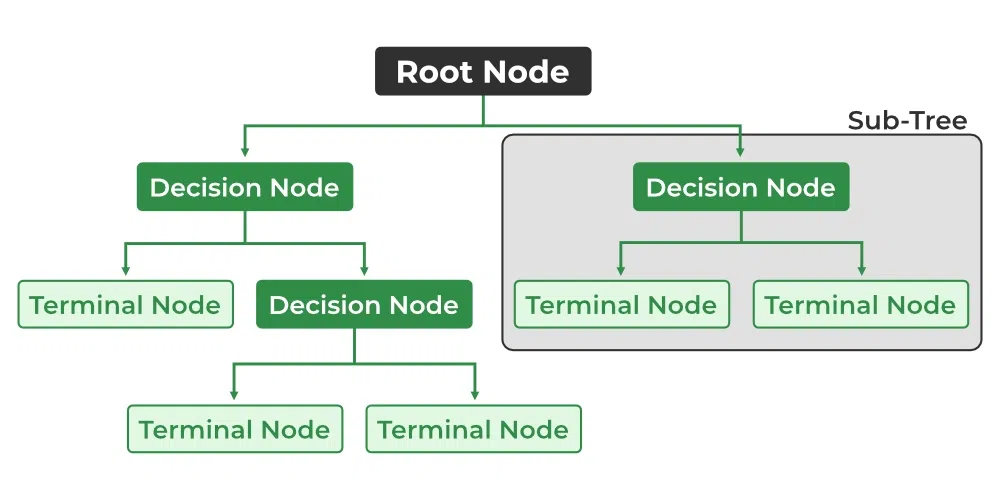
• Root Node: It is the topmost node in the tree,  which represents the complete dataset. It is the starting point of the decision-making process.
• Decision/Internal Node: A node that symbolizes a choice regarding an input feature. Branching off of internal nodes connects them to leaf nodes or other internal nodes.
• Leaf/Terminal Node: A node without any child nodes that indicates a class label or a numerical value.
• Splitting: The process of splitting a node into two or more sub-nodes using a split criterion and a selected feature.
• Branch/Sub-Tree: A subsection of the decision tree starts at an internal node and ends at the leaf nodes.
• Parent Node: The node that divides into one or more child nodes.
• Child Node: The nodes that emerge when a parent node is split.
• Impurity: A measurement of the target variable’s homogeneity in a subset of data. It refers to the degree of randomness or uncertainty in a set of examples. The Gini index and entropy are two commonly used impurity measurements in decision trees for classifications task 
• Variance: Variance measures how much the predicted and the target variables vary in different samples of a dataset. It is used for regression problems in decision trees. Mean squared error, Mean Absolute Error, friedman_mse, or Half Poisson deviance are used to measure the variance for the regression tasks in the decision tree.
• Information Gain: Information gain is a measure of the reduction in impurity achieved by splitting a dataset on a particular feature in a decision tree. The splitting criterion is determined by the feature that offers the greatest information gain, It is used to determine the most informative feature to split on at each node of the tree, with the goal of creating pure subsets
• Pruning: The process of removing branches from the tree that do not provide any additional information or lead to overfitting.

Decision Tree

Attribute Selection Measures:

Construction of Decision Tree: A tree can be “learned” by splitting the source set into subsets based on Attribute Selection Measures. Attribute selection measure (ASM) is a criterion used in decision tree algorithms to evaluate the usefulness of different attributes for splitting a dataset. The goal of ASM is to identify the attribute that will create the most homogeneous subsets of data after the split, thereby maximizing the information gain. This process is repeated on each derived subset in a recursive manner called recursive partitioning. The recursion is completed when the subset at a node all has the same value of the target variable, or when splitting no longer adds value to the predictions. The construction of a decision tree classifier does not require any domain knowledge or parameter setting and therefore is appropriate for exploratory knowledge discovery. Decision trees can handle high-dimensional data.

Entropy:

Entropy is the measure of the degree of randomness or uncertainty in the dataset. In the case of classifications, It measures the randomness based on the distribution of class labels in the dataset.

The entropy for a subset of the original dataset having K number of classes for the i^th node can be defined as:

Where,

• S is the dataset sample.
• k is the particular class from K classes
• p(k) is the proportion of the data points that belong to class k to the total number of data points in dataset sample S. 
• Here p(i,k) should not be equal to zero.

Important points related to Entropy:

1. The entropy is 0 when the dataset is completely homogeneous, meaning that each instance belongs to the same class. It is the lowest entropy indicating no uncertainty in the dataset sample.
2. when the dataset is equally divided between multiple classes, the entropy is at its maximum value. Therefore, entropy is highest when the distribution of class labels is even, indicating maximum uncertainty in the dataset sample.
3. Entropy is used to evaluate the quality of a split. The goal of entropy is to select the attribute that minimizes the entropy of the resulting subsets, by splitting the dataset into more homogeneous subsets with respect to the class labels.
4. The highest information gain attribute is chosen as the splitting criterion (i.e., the reduction in entropy after splitting on that attribute), and the process is repeated recursively to build the decision tree.

Gini Impurity or index:

Gini Impurity is a score that evaluates how accurate a split is among the classified groups. The Gini Impurity evaluates a score in the range between 0 and 1, where 0 is when all observations belong to one class, and 1 is a random distribution of the elements within classes. In this case, we want to have a Gini index score as low as possible. Gini Index is the evaluation metric we shall use to evaluate our Decision Tree Model.

Here,

• p_i is the proportion of elements in the set that belongs to the i^th category.

Information Gain:

Information gain measures the reduction in entropy or variance that results from splitting a dataset based on a specific property. It is used in decision tree algorithms to determine the usefulness of a feature by partitioning the dataset into more homogeneous subsets with respect to the class labels or target variable. The higher the information gain, the more valuable the feature is in predicting the target variable. 

The information gain of an attribute A, with respect to a dataset S, is calculated as follows:

where

• A is the specific attribute or class label
• |H| is the entropy of dataset sample S
• |H_V| is the number of instances in the subset S that have the value v for attribute A

Information gain measures the reduction in entropy or variance achieved by partitioning the dataset on attribute A. The attribute that maximizes information gain is chosen as the splitting criterion for building the decision tree.

Information gain is used in both classification and regression decision trees. In classification, entropy is used as a measure of impurity, while in regression, variance is used as a measure of impurity. The information gain calculation remains the same in both cases, except that entropy or variance is used instead of entropy in the formula.

Classification and Regression Tree algorithm

To build the Decision Tree, CART (Classification and Regression Tree) algorithm is used. It works by selecting the best split at each node based on metrics like Gini impurity or information Gain. In order to create a decision tree. Here are the basic steps of the CART algorithm:

1. The root node of the tree is supposed to be the complete training dataset.
2. Determine the impurity of the data based on each feature present in the dataset. Impurity can be measured using metrics like the Gini index or entropy for classification and Mean squared error, Mean Absolute Error, friedman_mse, or Half Poisson deviance for regression.
3. Then selects the feature that results in the highest information gain or impurity reduction when splitting the data.
4. For each possible value of the selected feature, split the dataset into two subsets (left and right), one where the feature takes on that value, and another where it does not. The split should be designed to create subsets that are as pure as possible with respect to the target variable.
5. Based on the target variable, determine the impurity of each resulting subset.
6. For each subset, repeat steps 2–5 iteratively until a stopping condition is met. For example, the stopping condition could be a maximum tree depth, a minimum number of samples required to make a split or a minimum impurity threshold.
7. Assign the majority class label for classification tasks or the mean value for regression tasks for each terminal node (leaf node) in the tree.

Classification and Regression Tree algorithm for Classification

Let the data available at node m be Q_m and it has n_m samples. and t_m as the threshold for node m. then, The classification and regression tree algorithm for classification can be written as :

Here,

• H is the measure of impurities of the left and right subsets at node m. it can be entropy or Gini impurity. 
• n_m is the number of instances in the left and right subsets at node m.

To select the parameter, we can write as:

Example:

Python3

# Import the necessary libraries
from sklearn.datasets import load_iris
from sklearn.tree import DecisionTreeClassifier
from sklearn.tree import export_graphviz
from graphviz import Source

# Load the dataset
iris = load_iris()
X = iris.data[:, 2:] # petal length and width
y = iris.target

# DecisionTreeClassifier
tree_clf = DecisionTreeClassifier(criterion='entropy',
                                  max_depth=2)
tree_clf.fit(X, y)

# Plot the decision tree graph
export_graphviz(
    tree_clf,
    out_file="iris_tree.dot",
    feature_names=iris.feature_names[2:],
    class_names=iris.target_names,
    rounded=True,
    filled=True
 )

with open("iris_tree.dot") as f:
    dot_graph = f.read()

Source(dot_graph)

Output:

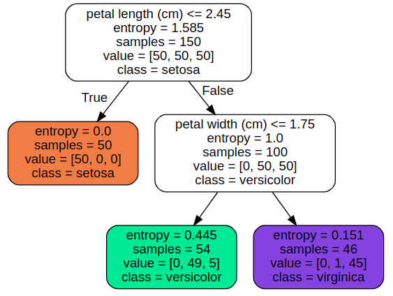
Decision Tree Classifier

Classification and Regression Tree algorithm for Regression

Let the data available at node m be Q_m and it has n_m samples. and t_m as the threshold for node m. then, The classification and regression tree algorithm for regression can be written as :

Here,

• MSE is the mean squared error.  
• n_m is the number of instances in the left and right subsets at node m.

To select the parameter, we can write as:

Example:

Python3

# Import the necessary libraries
from sklearn.datasets import load_diabetes
from sklearn.tree import DecisionTreeRegressor
from sklearn.tree import export_graphviz
from graphviz import Source

# Load the dataset
diabetes = load_diabetes()
X = diabetes.data
y = diabetes.target

# DecisionTreeRegressor
tree_reg = DecisionTreeRegressor(criterion = 'squared_error',
                                 max_depth=2)

tree_reg.fit(X, y)

# Plot the decision tree graph
export_graphviz(
    tree_reg,
    out_file="diabetes_tree.dot",
    feature_names=diabetes.feature_names,
    class_names=diabetes.target,
    rounded=True,
    filled=True
 )

with open("diabetes_tree.dot") as f:
    dot_graph = f.read()

Source(dot_graph)

Output:

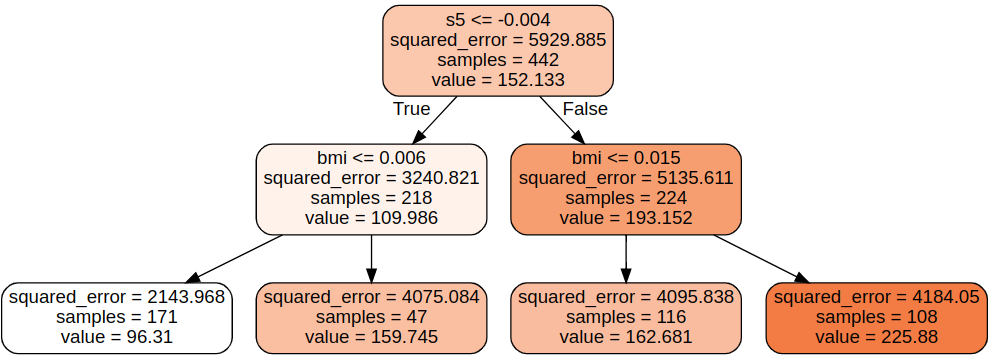
Decision Tree Regression

Strengths and Weaknesses of the Decision Tree Approach

The strengths of decision tree methods are: 

• Decision trees are able to generate understandable rules.
• Decision trees perform classification without requiring much computation.
• Decision trees are able to handle both continuous and categorical variables.
• Decision trees provide a clear indication of which fields are most important for prediction or classification.
• Ease of use: Decision trees are simple to use and don’t require a lot of technical expertise, making them accessible to a wide range of users.
• Scalability: Decision trees can handle large datasets and can be easily parallelized to improve processing time.
• Missing value tolerance: Decision trees are able to handle missing values in the data, making them a suitable choice for datasets with missing or incomplete data.
• Handling non-linear relationships: Decision trees can handle non-linear relationships between variables, making them a suitable choice for complex datasets.
• Ability to handle imbalanced data: Decision trees can handle imbalanced datasets, where one class is heavily represented compared to the others, by weighting the importance of individual nodes based on the class distribution.

The weaknesses of decision tree methods : 

• Decision trees are less appropriate for estimation tasks where the goal is to predict the value of a continuous attribute.
• Decision trees are prone to errors in classification problems with many classes and a relatively small number of training examples.
• Decision trees can be computationally expensive to train. The process of growing a decision tree is computationally expensive. At each node, each candidate splitting field must be sorted before its best split can be found. In some algorithms, combinations of fields are used and a search must be made for optimal combining weights. Pruning algorithms can also be expensive since many candidate sub-trees must be formed and compared.
• Decision trees are prone to overfitting the training data, particularly when the tree is very deep or complex. This can result in poor performance on new, unseen data.
• Small variations in the training data can result in different decision trees being generated, which can be a problem when trying to compare or reproduce results.
• Many decision tree algorithms do not handle missing data well, and require imputation or deletion of records with missing values.
• The initial splitting criteria used in decision tree algorithms can lead to biased trees, particularly when dealing with unbalanced datasets or rare classes.
• Decision trees are limited in their ability to represent complex relationships between variables, particularly when dealing with nonlinear or interactive effects.
• Decision trees can be sensitive to the scaling of input features, particularly when using distance-based metrics or decision rules that rely on comparisons between values.

Implementation:

C++

// Importing required headers
#include <algorithm>
#include <chrono>
#include <cmath>
#include <cstdlib>
#include <ctime>
#include <fstream>
#include <iostream>
#include <iterator>
#include <queue>
#include <random>
#include <sstream>
#include <vector>

#include <bits/stdc++.h>
#include <stdio.h>

using namespace std;

int main()
{
    // Generating random data for classification
    int X[100][5];
    int t[100];
    srand(10);
    for (int i = 0; i < 100; i++) {
        for (int j = 0; j < 5; j++) {
            X[i][j] = rand() % 2;
        }
        t[i] = rand() % 2;
    } // Splitting data into train and test sets
    int X_train[70][5];
    int X_test[30][5];
    int t_train[70];
    int t_test[30];

    for (int i = 0; i < 70; i++) {
        for (int j = 0; j < 5; j++) {
            X_train[i][j] = X[i][j];
        }
        t_train[i] = t[i];
    }

    for (int i = 0; i < 30; i++) {
        for (int j = 0; j < 5; j++) {
            X_test[i][j] = X[i + 70][j];
        }
        t_test[i] = t[i + 70];
    }

    // Randomly predicting binary values for test set
    int predicted_value[30];
    for (int i = 0; i < 30; i++) {
        predicted_value[i] = rand() % 2;
    }

    // Printing predicted binary values for test set
    for (int i = 0; i < 30; i++) {
        cout << predicted_value[i] << " ";
    }
    cout << "\n";

    // Calculating number of 0s and 1s in train set
    int zeroes = 0;
    int ones = 0;
    for (int i = 0; i < 70; i++) {
        if (t_train[i] == 0) {
            zeroes += 1;
        }
        else {
            ones += 1;
        }
    }

    // Calculating Gini index
    float val = 1
                - ((zeroes / 70.0) * (zeroes / 70.0)
                   + (ones / 70.0) * (ones / 70.0));
    cout << "Gini : " << val << "\n";

    // Calculating accuracy of predictions
    int match = 0;
    int UnMatch = 0;
    for (int i = 0; i < 30; i++) {
        if (predicted_value[i] == t_test[i]) {
            match += 1;
        }
        else {
            UnMatch += 1;
        }
    }
    float accuracy = match / 30.0;
    cout << "Accuracy is: " << accuracy << "\n";

    // Returning 0 on successful completion
    return 0;
}

Java

import java.util.Random;

public class Main {
    public static void main(String[] args) {
        // Generating random data for classification
        int[][] X = new int[100][5];
        int[] t = new int[100];
        Random rand = new Random(10);
        for (int i = 0; i < 100; i++) {
            for (int j = 0; j < 5; j++) {
                X[i][j] = rand.nextInt(2);
            }
            t[i] = rand.nextInt(2);
        }

        // Splitting data into train and test sets
        int[][] X_train = new int[70][5];
        int[][] X_test = new int[30][5];
        int[] t_train = new int[70];
        int[] t_test = new int[30];

        for (int i = 0; i < 70; i++) {
            for (int j = 0; j < 5; j++) {
                X_train[i][j] = X[i][j];
            }
            t_train[i] = t[i];
        }

        for (int i = 0; i < 30; i++) {
            for (int j = 0; j < 5; j++) {
                X_test[i][j] = X[i + 70][j];
            }
            t_test[i] = t[i + 70];
        }

        // Randomly predicting binary values for test set
        int[] predicted_value = new int[30];
        for (int i = 0; i < 30; i++) {
            predicted_value[i] = rand.nextInt(2);
        }

        // Printing predicted binary values for test set
        for (int i = 0; i < 30; i++) {
            System.out.print(predicted_value[i] + " ");
        }
        System.out.println();

        // Calculating number of 0s and 1s in train set
        int zeroes = 0;
        int ones = 0;
        for (int i = 0; i < 70; i++) {
            if (t_train[i] == 0) {
                zeroes += 1;
            }
            else {
                ones += 1;
            }
        }

        // Calculating Gini index
        float val = 1 - ((zeroes / 70.0f) * (zeroes / 70.0f) + (ones / 70.0f) * (ones / 70.0f));
        System.out.println("Gini : " + val);

        // Calculating accuracy of predictions
        int match = 0;
        int unMatch = 0;
        for (int i = 0; i < 30; i++) {
            if (predicted_value[i] == t_test[i]) {
                match += 1;
            }
            else {
                unMatch += 1;
            }
        }
        float accuracy = match / 30.0f;
        System.out.println("Accuracy is: " + accuracy);
    }
}

Python3

from sklearn.datasets import make_classification
from sklearn import tree
from sklearn.model_selection import train_test_split

X, t = make_classification(100, 5, n_classes=2, shuffle=True, random_state=10)
X_train, X_test, t_train, t_test = train_test_split(
    X, t, test_size=0.3, shuffle=True, random_state=1)

model = tree.DecisionTreeClassifier()
model = model.fit(X_train, t_train)

predicted_value = model.predict(X_test)
print(predicted_value)

tree.plot_tree(model)

zeroes = 0
ones = 0
for i in range(0, len(t_train)):
    if t_train[i] == 0:
        zeroes += 1
    else:
        ones += 1

print(zeroes)
print(ones)

val = 1 - ((zeroes/70)*(zeroes/70) + (ones/70)*(ones/70))
print("Gini :", val)

match = 0
UnMatch = 0

for i in range(30):
    if predicted_value[i] == t_test[i]:
        match += 1
    else:
        UnMatch += 1

accuracy = match/30
print("Accuracy is: ", accuracy)

C#

using System;
using System.Linq;

namespace ConsoleApp
{
    class Program
    {
        static void Main(string[] args)
        {
            // Generating random data for classification
            int[,] X = new int[100, 5];
            int[] t = new int[100];
            Random rand = new Random(10);
            for (int i = 0; i < 100; i++)
            {
                for (int j = 0; j < 5; j++)
                {
                    X[i, j] = rand.Next(0, 2);
                }
                t[i] = rand.Next(0, 2);
            }

            // Splitting data into train and test sets
            int[,] X_train = new int[70, 5];
            int[,] X_test = new int[30, 5];
            int[] t_train = new int[70];
            int[] t_test = new int[30];

            for (int i = 0; i < 70; i++)
            {
                for (int j = 0; j < 5; j++)
                {
                    X_train[i, j] = X[i, j];
                }
                t_train[i] = t[i];
            }

            for (int i = 0; i < 30; i++)
            {
                for (int j = 0; j < 5; j++)
                {
                    X_test[i, j] = X[i + 70, j];
                }
                t_test[i] = t[i + 70];
            }

            // Randomly predicting binary values for test set
            int[] predicted_value = new int[30];
            for (int i = 0; i < 30; i++)
            {
                predicted_value[i] = rand.Next(0, 2);
            }

            // Printing predicted binary values for test set
            Console.WriteLine(String.Join(" ", predicted_value));

            // Calculating number of 0s and 1s in train set
            int zeroes = t_train.Count(x => x == 0);
            int ones = t_train.Count(x => x == 1);

            // Calculating Gini index
            float val = 1
                        - ((zeroes / 70.0f) * (zeroes / 70.0f)
                           + (ones / 70.0f) * (ones / 70.0f));
            Console.WriteLine("Gini : " + val);

            // Calculating accuracy of predictions
            int match = 0;
            int UnMatch = 0;
            for (int i = 0; i < 30; i++)
            {
                if (predicted_value[i] == t_test[i])
                {
                    match += 1;
                }
                else
                {
                    UnMatch += 1;
                }
            }
            float accuracy = match / 30.0f;
            Console.WriteLine("Accuracy is: " + accuracy);

            // Returning 0 on successful completion
            Environment.Exit(0);
        }
    }
}
//this code is added snehalsalokhe

Javascript

// Generating random data for classification
let X = Array.from(Array(100), () => new Array(5));
let t = new Array(100);
for (let i = 0; i < 100; i++) {
    for (let j = 0; j < 5; j++) {
        X[i][j] = Math.floor(Math.random() * 2);
    }
    t[i] = Math.floor(Math.random() * 2);
}

// Splitting data into train and test sets
let X_train = Array.from(Array(70), () => new Array(5));
let X_test = Array.from(Array(30), () => new Array(5));
let t_train = new Array(70);
let t_test = new Array(30);

for (let i = 0; i < 70; i++) {
    for (let j = 0; j < 5; j++) {
        X_train[i][j] = X[i][j];
    }
    t_train[i] = t[i];
}

for (let i = 0; i < 30; i++) {
    for (let j = 0; j < 5; j++) {
        X_test[i][j] = X[i + 70][j];
    }
    t_test[i] = t[i + 70];
}

// Randomly predicting binary values for test set
let predicted_value = new Array(30);
for (let i = 0; i < 30; i++) {
    predicted_value[i] = Math.floor(Math.random() * 2);
}

// Printing predicted binary values for test set
for (let i = 0; i < 30; i++) {
    process.stdout.write(predicted_value[i] + " ");
}
console.log();

// Calculating number of 0s and 1s in train set
let zeroes = 0;
let ones = 0;
for (let i = 0; i < 70; i++) {
    if (t_train[i] == 0) {
        zeroes += 1;
    } else {
        ones += 1;
    }
}

// Calculating Gini index
let val =
    1 -
    (zeroes / 70.0) * (zeroes / 70.0) -
    (ones / 70.0) * (ones / 70.0);
console.log("Gini : " + val);

// Calculating accuracy of predictions
let match = 0;
let UnMatch = 0;
for (let i = 0; i < 30; i++) {
    if (predicted_value[i] == t_test[i]) {
        match += 1;
    } else {
        UnMatch += 1;
    }
}
let accuracy = match / 30.0;
console.log("Accuracy is: " + accuracy);

Output

1 1 0 0 1 0 1 0 1 0 0 1 1 0 0 1 0 1 1 1 0 0 0 1 1 0 0 0 1 0 
Gini : 0.5
Accuracy is: 0.366667

In the next post, we will be discussing the ID3 algorithm for the construction of the Decision tree given by J. R. Quinlan.