Data Processing is an important part of any task that includes data-driven work. It helps us to provide meaningful insights from the data. As we know Python is a widely used programming language, and there are various libraries and tools available for data processing.
In this article, we are going to see Data Processing in Python, Loading, Printing rows and Columns, Data frame summary, Missing data values Sorting and Merging Data Frames, Applying Functions, and Visualizing Dataframes.
What is Data Processing in Python?
Data processing in Python refers to manipulating, transforming, and analyzing data by using Python. It contains a series of operations that aim to change raw data into structured data. or meaningful insights. By converting raw data into meaningful insights it makes it suitable for analysis, visualization, or other applications.Python provides several libraries and tools that facilitate efficient data processing, making it a popular choice for working with diverse datasets.
Refer to this article – Introduction to Data Processing
What is Pandas?
Pandas is a powerful, fast, and open-source library built on NumPy. It is used for data manipulation and real-world data analysis in Python. Easy handling of missing data, Flexible reshaping and pivoting of data sets, and size mutability make pandas a great tool for performing data manipulation and handling the data efficiently.
Loading Data in Pandas DataFrame
Reading CSV file using pd.read_csv and loading data into a data frame. Import pandas as using pd for the shorthand. You can download the data from here.
Python3
import pandas as pd
data_frame=pd.read_csv('Mall_Customers.csv')
|
Printing rows of the Data
By default, data_frame.head() displays the first five rows and data_frame.tail() displays last five rows. If we want to get first ‘n’ number of rows then we use, data_frame.head(n) similar is the syntax to print the last n rows of the data frame.
Python3
display(data_frame.head())
display(data_frame.tail())
|
Output:
   CustomerID   Genre  Age  Annual Income (k$)  Spending Score (1-100)
0           1    Male   19                  15                      39
1           2    Male   21                  15                      81
2           3  Female   20                  16                       6
3           4  Female   23                  16                      77
4           5  Female   31                  17                      40
     CustomerID   Genre  Age  Annual Income (k$)  Spending Score (1-100)
195         196  Female   35                 120                      79
196         197  Female   45                 126                      28
197         198    Male   32                 126                      74
198         199    Male   32                 137                      18
199         200    Male   30                 137                      83
[4]
0s
# Program to print all the column name of the dataframe
print(list(data_frame.columns))
Printing the column names of the DataFrame
Python3
print(list(data_frame.columns))
|
Output:
['CustomerID', 'Genre', 'Age', 'Annual Income (k$)', 'Spending Score (1-100)']
Summary of Data Frame
The functions info() prints the summary of a DataFrame that includes the data type of each column, RangeIndex (number of rows), columns, non-null values, and memory usage.
Output:
<class 'pandas.core.frame.DataFrame'>
RangeIndex: 200 entries, 0 to 199
Data columns (total 5 columns):
 #   Column                  Non-Null Count  Dtype
---  ------                  --------------  -----
 0   CustomerID              200 non-null    int64
 1   Genre                   200 non-null    object
 2   Age                     200 non-null    int64
 3   Annual Income (k$)      200 non-null    int64
 4   Spending Score (1-100)  200 non-null    int64
dtypes: int64(4), object(1)
memory usage: 7.9+ KB
Descriptive Statistical Measures of a DataFrame
The describe() function outputs descriptive statistics which include those that summarize the central tendency, dispersion, and shape of a dataset’s distribution, excluding NaN values. For numeric data, the result’s index will include count, mean, std, min, and max as well as lower, 50, and upper percentiles. For object data (e.g. strings), the result’s index will include count, unique, top, and freq.
Output:
       CustomerID         Age  Annual Income (k$)  Spending Score (1-100)
count  200.000000  200.000000          200.000000              200.000000
mean   100.500000   38.850000           60.560000               50.200000
std     57.879185   13.969007           26.264721               25.823522
min      1.000000   18.000000           15.000000                1.000000
25%     50.750000   28.750000           41.500000               34.750000
50%    100.500000   36.000000           61.500000               50.000000
75%    150.250000   49.000000           78.000000               73.000000
max    200.000000   70.000000          137.000000               99.000000
Missing Data Handing
Find missing values in the dataset
The isnull( ) detects the missing values and returns a boolean object indicating if the values are NA. The values which are none or empty get mapped to true values and not null values get mapped to false values.
Output:
     CustomerID  Genre    Age  Annual Income (k$)  Spending Score (1-100)
0         False  False  False               False                   False
1         False  False  False               False                   False
2         False  False  False               False                   False
3         False  False  False               False                   False
4         False  False  False               False                   False
..          ...    ...    ...                 ...                     ...
195       False  False  False               False                   False
196       False  False  False               False                   False
197       False  False  False               False                   False
198       False  False  False               False                   False
199       False  False  False               False                   False
[200 rows x 5 columns]
[8]
0s
Find the number of missing values in the dataset
To find out the number of missing values in the dataset, use data_frame.isnull( ).sum( ). In the below example, the dataset doesn’t contain any null values. Hence, each column’s output is 0.
Python3
data_frame.isnull().sum()
|
Output:
CustomerID                0
Genre                     0
Age                       0
Annual Income (k$)        0
Spending Score (1-100)    0
dtype: int64
Removing missing values
The data_frame.dropna( ) function removes columns or rows which contains atleast one missing values.
data_frame = data_frame.dropna()
By default, data_frame.dropna( ) drops the rows where at least one element is missing. data_frame.dropna(axis = 1) drops the columns where at least one element is missing.
Fill in missing values
We can fill null values using data_frame.fillna( ) function.
data_frame = data_frame.fillna(value)
But by using the above format all the null values will get filled with the same values. To fill different values in the different columns we can use.
data_frame[col] = data_frame[col].fillna(value)
Row and column manipulations
Removing rows
By using the drop(index) function we can drop the row at a particular index. If we want to replace the data_frame with the row removed then add inplace = True in the drop function.
Python3
data_frame.drop(4).head()
|
Output:
   CustomerID   Genre  Age  Annual Income (k$)  Spending Score (1-100)
0           1    Male   19                  15                      39
1           2    Male   21                  15                      81
2           3  Female   20                  16                       6
3           4  Female   23                  16                      77
5           6  Female   22                  17                      76
[ ]
This function can also be used to remove the columns of a data frame by adding the attribute axis =1 and providing the list of columns we would like to remove.
Renaming rows
The rename function can be used to rename the rows or columns of the data frame.
Python3
data_frame.rename({0:"First",1:"Second"})
|
Output:
        CustomerID   Genre  Age  Annual Income (k$)  Spending Score (1-100)
First            1    Male   19                  15                      39
Second           2    Male   21                  15                      81
2                3  Female   20                  16                       6
3                4  Female   23                  16                      77
4                5  Female   31                  17                      40
...            ...     ...  ...                 ...                     ...
195            196  Female   35                 120                      79
196            197  Female   45                 126                      28
197            198    Male   32                 126                      74
198            199    Male   32                 137                      18
199            200    Male   30                 137                      83
[200 rows x 5 columns]
Adding new columns
Python3
data_frame['NewColumn'] = 1
data_frame.head()
|
Output:
   CustomerID   Genre  Age  Annual Income (k$)  Spending Score (1-100)  \
0           1    Male   19                  15                      39
1           2    Male   21                  15                      81
2           3  Female   20                  16                       6
3           4  Female   23                  16                      77
4           5  Female   31                  17                      40
   NewColumn
0          1
1          1
2          1
3          1
4          1
Sorting DataFrame values
Sort by column
The sort_values( ) are the values of the column whose name is passed in the by attribute in the ascending order by default we can set this attribute to false to sort the array in the descending order.
Python3
data_frame.sort_values(by='Age', ascending=False).head()
|
Output:
    CustomerID   Genre  Age  Annual Income (k$)  Spending Score (1-100)  \
70          71    Male   70                  49                      55
60          61    Male   70                  46                      56
57          58    Male   69                  44                      46
90          91  Female   68                  59                      55
67          68  Female   68                  48                      48
    NewColumn
70          1
60          1
57          1
90          1
67          1
Sort by multiple columns
Python3
data_frame.sort_values(by=['Age','Annual Income (k$)']).head(10)
|
Output:
     CustomerID   Genre  Age  Annual Income (k$)  Spending Score (1-100)  \
33           34    Male   18                  33                      92
65           66    Male   18                  48                      59
91           92    Male   18                  59                      41
114         115  Female   18                  65                      48
0             1    Male   19                  15                      39
61           62    Male   19                  46                      55
68           69    Male   19                  48                      59
111         112  Female   19                  63                      54
113         114    Male   19                  64                      46
115         116  Female   19                  65                      50
     NewColumn
33           1
65           1
91           1
114          1
0            1
61           1
68           1
111          1
113          1
115          1
Merge Data Frames
The merge() function in pandas is used for all standard database join operations. Merge operation on data frames will join two data frames based on their common column values. Let’s create a data frame.
Python3
df1 = pd.DataFrame({
'Name':['Jeevan', 'Raavan', 'Geeta', 'Bheem'],
'Age':[25, 24, 52, 40],
'Qualification':['Msc', 'MA', 'MCA', 'Phd']})
df1
|
Output:
     Name  Age Qualification
0  Jeevan   25           Msc
1  Raavan   24            MA
2   Geeta   52           MCA
3   Bheem   40           Phd
Now we will create another data frame.
Python3
df2 = pd.DataFrame({'Name':['Jeevan', 'Raavan', 'Geeta', 'Bheem'],
'Salary':[100000, 50000, 20000, 40000]})
df2
|
Output:
     Name  Salary
0  Jeevan  100000
1  Raavan   50000
2   Geeta   20000
3   Bheem   40000
Now. let’s merge these two data frames created earlier.
Python3
df = pd.merge(df1, df2)
df
|
Output:
     Name  Age Qualification  Salary
0  Jeevan   25           Msc  100000
1  Raavan   24            MA   50000
2   Geeta   52           MCA   20000
3   Bheem   40           Phd   40000
Apply Function
By defining a function beforehand
The apply( ) function is used to iterate over a data frame. It can also be used with lambda functions.
Python3
def fun(value):
if value > 70:
return "Yes"
else:
return "No"
data_frame['Customer Satisfaction'] = data_frame['Spending Score (1-100)'].apply(fun)
data_frame.head(10)
|
Output:
   CustomerID   Genre  Age  Annual Income (k$)  Spending Score (1-100)  \
0           1    Male   19                  15                      39
1           2    Male   21                  15                      81
2           3  Female   20                  16                       6
3           4  Female   23                  16                      77
4           5  Female   31                  17                      40
5           6  Female   22                  17                      76
6           7  Female   35                  18                       6
7           8  Female   23                  18                      94
8           9    Male   64                  19                       3
9          10  Female   30                  19                      72
   NewColumn Customer Satisfaction
0          1                    No
1          1                   Yes
2          1                    No
3          1                   Yes
4          1                    No
5          1                   Yes
6          1                    No
7          1                   Yes
8          1                    No
9          1                   Yes
By using the lambda operator
This syntax is generally used to apply log transformations and normalize the data to bring it in the range of 0 to 1 for particular columns of the data.
Python3
const = data_frame['Age'].max()
data_frame['Age'] = data_frame['Age'].apply(lambda x: x/const)
data_frame.head()
|
Output:
   CustomerID   Genre       Age  Annual Income (k$)  Spending Score (1-100)  \
0           1    Male  0.271429                  15                      39
1           2    Male  0.300000                  15                      81
2           3  Female  0.285714                  16                       6
3           4  Female  0.328571                  16                      77
4           5  Female  0.442857                  17                      40
   NewColumn Customer Satisfaction
0          1                    No
1          1                   Yes
2          1                    No
3          1                   Yes
4          1                    No
Visualizing DataFrame
Scatter plot
The plot( ) function is used to make plots of the data frames.
Python3
data_frame.plot(x ='CustomerID', y='Spending Score (1-100)',kind = 'scatter')
|
Output:
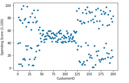
Scatter plot of the Customer Satisfaction column
Histogram
The plot.hist( ) function is used to make plots of the data frames.
Output:
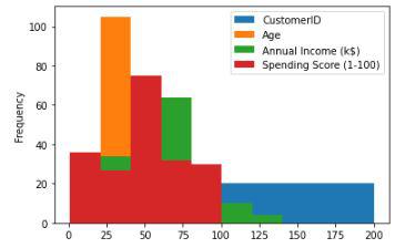
Histogram for the distribution of the data
Conclusion
There are other functions as well of pandas data frame but the above mentioned are some of the common ones generally used for handling large tabular data. One can refer to the pandas documentation as well to explore more about the functions mentioned above.
Share your thoughts in the comments
Please Login to comment...