Benchmarking in Julia
Last Updated :
03 Aug, 2021
In Julia, most of the codes are checked for it’s speed and efficiency. One of the hallmarks of Julia is that it’s quite faster than it’s other scientific computing counterparts(Python, R, Matlab). To verify this, we often tend to compare the speed and performance of a code block run across various languages. In cases where we try out multiple methods to solve a problem, and it becomes necessary to decide the most efficient approach, in that case we obviously choose the fastest method.
One of the most conventional ways to test out a code block in Julia is using the @time macro. In Julia we say that global objects tend to decrease performance.
Also, since we use randomly generated values, we will seed the RNG, so that the values are consistent between trials/samples/evaluations.
Python3
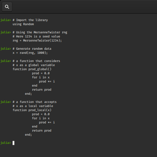
using Random
rng = MersenneTwister(1234);
x = rand(rng, 1000);
function prod_global()
prod = 0.0
for i in x
prod *= i
end
return prod
end;
function prod_local(x)
prod = 0.0
for i in x
prod *= i
end
return prod
end;
|
Output:
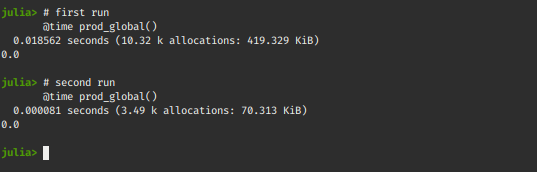
Now to compare the two functions we will use our @time macro. For a fresh environment, on the first call (@time prod_global()), the prod_global() function and other functions needed for timing are compiled so the results of first run shouldn’t be taken seriously.
Python3
@time prod_global()
@time prod_global()
|
Output:
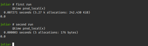
Let’s try to test the function with a local x
Python3
@time prod_local(x)
@time prod_local(x)
|
Output:
Profiling Julia Code
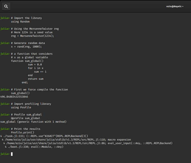
For profiling code in Julia we use the @profile macro. It performs measurements on running code, and produces output that helps developers analyze the time spent per line. It is generally used to identify bottlenecks in code blocks/functions that hinder performance.
Let’s try to profile our previous example and see why global variables hinder performance!
Also, we will replace the product by sum now, so that the calculations don’t tend towards infinity or zero at any point.
Python3
using Random
rng = MersenneTwister(1234);
x = rand(rng, 1000);
function sum_global()
sum = 0.0
for i in x
sum += i
end
return sum
end;
sum_global()
using Profile
@profile sum_global
Profile.print()
|
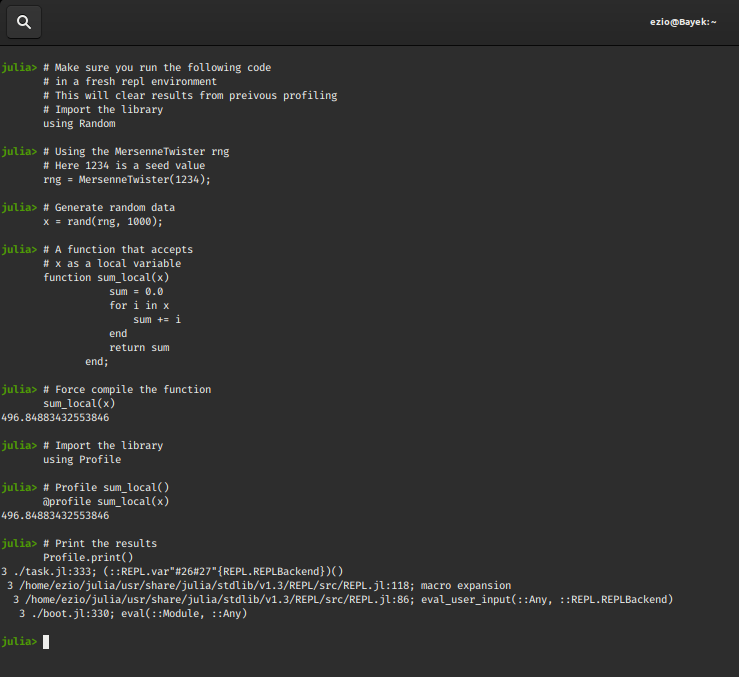
Output:
Python3
using Random
rng = MersenneTwister(1234);
x = rand(rng, 1000);
function sum_local(x)
sum = 0.0
for i in x
sum += i
end
return sum
end;
sum_local(x)
using Profile
@profile sum_local(x)
Profile.print()
|
Output:
You must be wondering that how can we simply conclude the performance of a code based on @time and profiling on one go and many of such decisions are made by consistent analysis across various trials and observing the code block’s performance over time. Julia has an extension package to run reliable benchmarks called Benchmark Tools.jl
Benchmarking a Code
One of the most conventional ways to benchmark a code block using Benchmark Tools is the @benchmark macro
Considering the above example of sum_local(x) and sum_global():
Python3
using Random
rng = MersenneTwister(1234);
using BenchmarkTools
x = rand(rng, 1000);
function sum_global()
sum = 0.0
for i in x
sum += i
end
return sum
end;
function sum_local(x)
sum = 0.0
for i in x
sum += i
end
return sum
end;
@benchmark sum_global()
@benchmark sum_local(x)
|
Output:
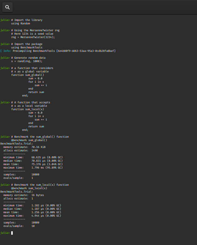
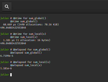
The @benchmark macro gives out a lot of details(mem. allocs, minimum time, mean time, median time, samples etc.) that come in handy for many developers, but there are times when we need a quick specific reference, eg : the @btime macro prints the minimum time and memory allocation before returning the value of the expression and the @belapsed macro returns the minimum time in seconds.
Python3
@btime sum_global()
@btime sum_local(x)
@belapsed sum_global()
@belapsed sum_local(x)
|
Output:
The @benchmark macro offers us ways to configure the benchmark process.
You can pass the following keyword arguments to @benchmark, and run to configure the execution process:
- samples: It determines the number of samples to take and defaults to
BenchmarkTools.DEFAULT_PARAMETERS.samples = 10000.
- seconds: The number of seconds allocated for the benchmarking process. The trial will terminate if this time is exceeded irrespective of number of samples, but atleast one sample will always be taken.
It defaults to BenchmarkTools.DEFAULT_PARAMETERS.seconds = 5.
- evals: It determines the number of evaluations per sample. It defaults to
BenchmarkTools.DEFAULT_PARAMETERS.evals = 1.
- overhead: The estimated loop overhead per evaluation in nanoseconds, which is automatically subtracted from every sample time measurement. The default value is
BenchmarkTools.DEFAULT_PARAMETERS.overhead = 0
- gctrial: If true, run gc() (garbage collector)before executing the benchmark’s trial.
Defaults to BenchmarkTools.DEFAULT_PARAMETERS.gctrial = true.
- gcsample: If set true, run gc() before each sample.
Defaults to BenchmarkTools.DEFAULT_PARAMETERS.gcsample = false.
- time_tolerance: The noise tolerance for the benchmark’s time estimate, as a percentage. This is utilized after benchmark execution, when analyzing results.
Defaults to BenchmarkTools.DEFAULT_PARAMETERS.time_tolerance = 0.05.
- memory_tolerance: The noise tolerance for the benchmark’s memory estimate, as a percentage. This is utilized after benchmark execution, when analyzing results.
Defaults to BenchmarkTools.DEFAULT_PARAMETERS.memory_tolerance = 0.01.
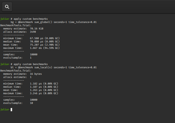
Python3
bg = @benchmark sum_global() seconds=1 time_tolerance=0.01
bl = @benchmark sum_local(x) seconds=1 time_tolerance=0.01
|
Output:
Share your thoughts in the comments
Please Login to comment...