Basic Operations in Octave

GNU Octave is a high-level programming language, primarily intended for numerical computations. It can also be used to implement various machine learning algorithms with ease. Octave is open-source i.e. it is free to use, whereas MATLAB is not thus MATLAB requires a license to operate.

Below are the various basic functionalities of Octave :

1. Arithmetic Operations : Octave can be used to perform basic mathematical operations like addition, subtraction, multiplication, power operation etc. 

MATLAB

% addition operation
23 + 65 + 8

% subtraction operation
32 - 74

% power operation
6 ^ 2

% multiplication operation
45 * 7

% division operation
5 / 6

Output : 

ans = 96
ans = -42
ans = 36
ans = 315
ans = 0.83333

2. Logical Operations : Octave can be used to perform logical operations like AND, OR, NOT etc. 

MATLAB

% logical AND
1 && 0

% logical OR
1 || 0

% logical NOT
~1

Output :

ans = 0
ans = 1
ans = 0

3. Relational Operations : Octave can be used to perform relational operations like greater than, less than etc.

MATLAB

% equal to
1 == 1

% not equal to
0 ~= 0

% greater than
1 > 0

% less than
1 < 0

% greater than equal to
1 >= 2

% less than equal to
0 <= 0

Output :

ans = 1
ans = 0
ans = 1
ans = 0
ans = 0
ans = 1

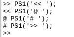
4. Changing the default Octave prompt symbol : The default Octave prompt symbol is “>>”. We can change the default Octave prompt symbol using the below commands :

MATLAB

PS1('<< ');
PS1('@ ');
PS1('# ');

Output :

5. Variables: Like other programming languages, Octave also has variables to temporarily store data.

MATLAB

% variable declaration and initialization
var = 2

% if we want to create the variable and don't want to print it
% then put a semicolon at the end of that command
var = 3; % this time the variable will not be printed

% variable of datatype char
ch = 'c'

% storing the result of an operation in a variable
res = (1 != 1)

% storing the value of pi in a variable
var = pi

% printing a variable with disp() function
disp(var);

% using sprintf() function to print a string
disp(sprintf('3 decimal values : %0.3f', var))

% using format long to resize
format long
var

% using format short to resize
format short
var

Output :

var =  2
ch = c
res = 0
var =  3.1416
 3.1416
3 decimal values : 3.142
var =  3.141592653589793
var =  3.1416

6. Matrices and Vectors: Now let’s learn how to deal with matrices and vectors in Octave. We can create matrix as shown below.

MATLAB

% creating matrix in row major
matrix = [1 2 3; 4 5 6; 7 8 9]

Output : 

matrix =

   1   2   3
   4   5   6
   7   8   9

We can also make a vector, a vector is a matrix with n rows and 1 column(column vector) or 1 rows with n columns(row vector). here in example 2 and 3 the middle value 5 and 0.5 shows that we want to make a vector matrix from range 1 to 20 with the jump of 5 and from range 0 to 5 with a jump of 0.5 respectively. 

MATLAB

% creating row vector
r_v = [1, 2, 3]

% creating column vector
c_v = [1; 2; 3]

Output : 

r_v =

   1   2   3

c_v =

   1
   2
   3

Here are some utility shortcuts to create matrices and vectors :

MATLAB

% creating vector using ":"
% the extreme end values denote the range
% and the middle value denotes the step
v1 = 1 : 5 : 20
v2 = 1 : 0.5 : 5

% without the step parameter
v3 = 1 : 10

% generate matrix of size 4x4 with all element as 1
ones_matrix = ones(4, 4)

% generate matrix of size 4x4 with all element as 10
M = 10 * ones(4, 4)

% generate row vector of size 5 with all elements 0
zeroes_vector = zeros(1, 5)

% generate row vector of some random numbers between 0 and 1
random_vector = rand(1, 5)

% generate matrix of some random numbers between 0 and 1
random_matrix = rand(3, 4)

% generate matrix with Gaussian distribution
% where mean = 0 and variance and standard deviation = 1
gauss_matrix = randn(5, 5)

% generate identity matrix with size 5x5
identity_matrix = eye(5)

Output : 

v1 =

    1    6   11   16

v2 =

    1.0000    1.5000    2.0000    2.5000    3.0000    3.5000    4.0000    4.5000    5.0000

v3 =

    1    2    3    4    5    6    7    8    9   10

ones_matrix =

   1   1   1   1
   1   1   1   1
   1   1   1   1
   1   1   1   1

M =

   10   10   10   10
   10   10   10   10
   10   10   10   10
   10   10   10   10

zeroes_vector =

   0   0   0   0   0

random_vector =

   0.79085   0.35395   0.92267   0.60234   0.75549

random_matrix =

   0.64434   0.67677   0.54105   0.83149
   0.70150   0.16149   0.38742   0.90442
   0.60075   0.82273   0.37113   0.91496

gauss_matrix =

   0.705921   1.336101  -0.097530   0.498245   1.125928
  -0.550047  -1.868716  -0.977788   0.319715  -0.603599
  -0.018352  -2.133200   0.462272   0.169707   1.733255
   0.623343   0.338734   0.618943   1.110172   1.731495
  -1.741052  -0.463446   0.556348   1.633956  -1.424136

identity_matrix =

Diagonal Matrix

   1   0   0   0   0
   0   1   0   0   0
   0   0   1   0   0
   0   0   0   1   0
   0   0   0   0   1

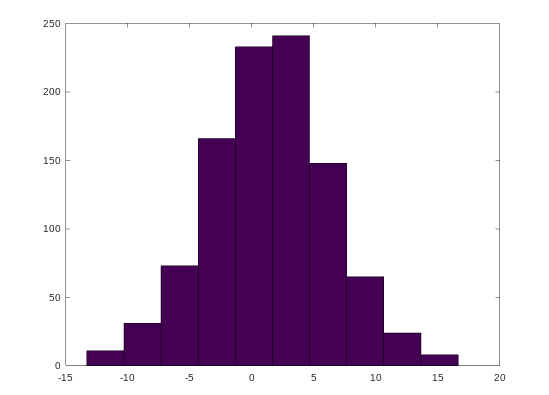
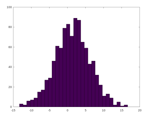
7. Histograms : We can draw the histograms hist() function. We can also change the bucket size or bins of the histogram.

MATLAB

% generate a vector with 1000 elements
elements_1000 = 1 + sqrt(25)*(randn(1, 1000));

hist(elements_1000 )

Output : 

MATLAB

% generate a vector with 1000 elements
elements_1000 = 1 + sqrt(25)*(randn(1, 1000));

% histogram with 30 bins
hist(elements_1000, 30)

Output : 

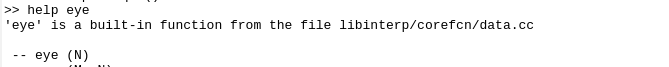
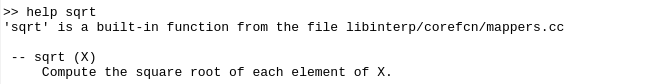
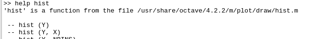
8. Help : We can use the help command to see the documentation for any function.  

MATLAB

help eye
help sqrt
help hist

Output :