Ball Tree and KD Tree Algorithms

Ball tree and KD-tree (K-Dimensional tree) are sophisticated data structures used in Python for efficiently organizing and searching multidimensional data. Imagine the ball tree algorithm as a way of grouping points into a tree structure by enclosing them within hyperspheres. This clever organization facilitates speedy searches for the nearest neighbors, making it particularly handy in machine-learning tasks like clustering and classification.

Now, the KD-tree algorithm takes a different approach. It partitions the data space using hyperplanes that are perpendicular to the coordinate axes, creating a binary tree structure. This characteristic makes KD-trees great for spatial indexing, and they are commonly used in algorithms where finding the nearest neighbors efficiently is crucial, such as in k-nearest neighbour (KNN) classification.

Ball Tree and KD Tree Algorithms

Both ball tree and KD-tree algorithms are implemented in Python libraries like Scikit-learn, giving users powerful tools to optimize nearest-neighbor search operations across various dimensions and dataset characteristics. When deciding between these algorithms, it often boils down to the specific needs and features of the data you’re working with.

KD Algorithm

A KD-tree (K-Dimensional tree) is a space-partitioning data structure that recursively subdivides a multidimensional space into regions associated with specific data points. The primary objective of a KD-tree is to facilitate efficient multidimensional search operations, particularly nearest-neighbor searches. The algorithm constructs a binary tree in which each node represents a region in the multidimensional space, and the associated hyperplane is aligned with one of the coordinate axes. At each level of the tree, the algorithm selects a dimension to split the data, creating two child nodes. This process continues recursively until a termination condition is met, such as a predefined depth or a threshold number of points per node. KD-trees are widely used in applications like k-nearest neighbor search, range queries, and spatial indexing, providing logarithmic time complexity for various search operations in average cases.

How KD Tree Alogrithm Works?

A data structure called a KD-tree (K-dimensional tree) is employed for effective multidimensional search processes. It generates a binary tree by recursively splitting the data along axes. The method divides the data into two subsets at each level according to the median value along a selected dimension. As a result of this ongoing process, a tree is formed, with each node representing a region in the multidimensional space. KD-trees reduce the search space through selected axis-aligned splits, allowing for quick closest neighbor searches and spatial queries that enable effective point retrieval in high-dimensional fields.

Example of KD Tree Algorithm

Let’s consider a simple real-world example to understand the concepts of KD-Tree algorithms:

Scenario: Finding Nearest Neighbors in a City

Imagine you are in a city and want to find the nearest coffee shop to your current location. The city is represented as a two-dimensional space where each point corresponds to a different location. The goal is to use spatial indexing algorithms to efficiently find the closest coffee shop.

In the KD-Tree approach, the city is divided into rectangular regions using perpendicular lines along the x and y axes. Each line represents a decision boundary based on the coordinates of the locations. For instance, if you decide to split along the x-axis first, the algorithm might create a vertical line that separates locations to the left and right. The process repeats recursively, creating a binary tree. When searching for the nearest coffee shop, the KD-Tree guides you efficiently through the tree, eliminating regions that cannot contain the closest shop and narrowing down the search space.

Diagram representing KD Tree Algorithm

Let’s see four coffee shops (A, B, C, and D) represented as points in a 2D space. The KD-Tree splits the space along the x and y axes.

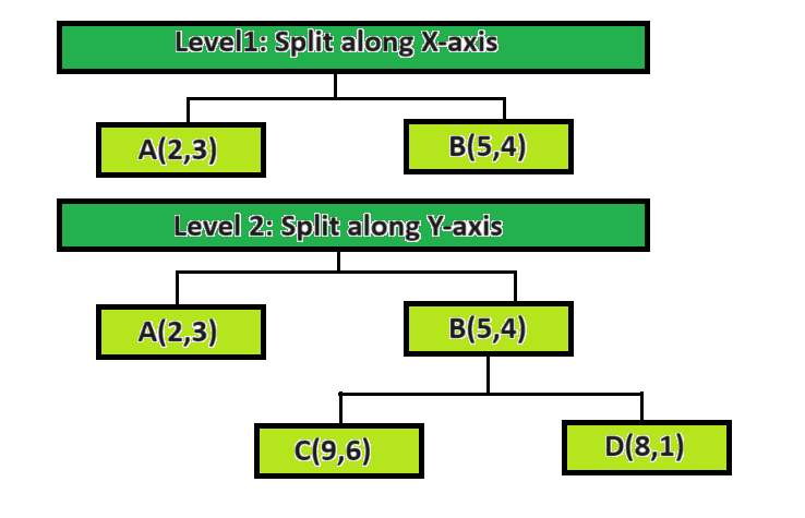
k-d tree algorithm

Now, if you’re looking for the nearest coffee shop to your location (let’s say, (3, 5)), the KD-Tree guides you through the search space efficiently by considering whether to go left or right based on the x and y axes.

Key Concepts of KD Tree Algorithm

Here are the key concepts related to the KD-tree algorithm:

1. Space Partitioning:

• Binary Tree Structure: The KD-tree organizes points in a multidimensional space into a binary tree. Each node in the tree represents a region in the space.
• Dimensional Splitting: At each level of the tree, the algorithm selects a dimension along which to split the data. This creates a hyperplane perpendicular to the chosen axis.

2. Recursive Construction: The process of constructing a KD-tree is recursive. At each level, the algorithm selects a dimension, finds the median value along that dimension, and splits the data into two subsets. This splitting process continues until a termination condition is met, such as a predefined depth or a minimum number of points per node.

3. Node Representation:

• Node Attributes: Each node in the KD-tree has attributes representing the dimension along which the data is split, the median value along that dimension, and pointers to the child nodes (left and right).
• Leaf Nodes: The terminal nodes of the tree are called leaf nodes and contain a subset of the data points.

4. Search Operations:

• Nearest Neighbor Search: KD-trees are often used for efficient nearest neighbor searches. During a search, the algorithm traverses the tree, eliminating subtrees based on distance metrics, and identifies the closest points.
• Range Queries: KD-trees can also be used for range queries, where all points within a certain distance from a query point are retrieved.

5. Balancing:

• Balanced Tree: Ideally, a balanced KD-tree minimizes the depth of the tree, ensuring efficient search times. However, balancing can be a challenging aspect of KD-tree construction.

6. Choice of Splitting Dimension:

• Coordinate Axis Selection: The algorithm must decide which dimension to split at each level. Common approaches include alternating dimensions or choosing the dimension with the maximum variance.

7. Applications:

• K-Nearest Neighbor Search: KD-trees are particularly popular for K-nearest neighbor (KNN) search algorithms.
• Spatial Indexing: KD-trees are used in spatial databases and Geographic Information Systems (GIS) for efficient data retrieval based on spatial proximity.

Understanding these concepts is crucial for effectively implementing and utilizing KD-trees in various applications involving multidimensional data. The choice of splitting dimension, balancing strategies, and termination conditions can impact the performance of the KD-tree algorithm in different scenarios.

Implementation of KD Tree Algorithm

Python3

from sklearn.neighbors import KDTree
import numpy as np

# Sample data
data = np.array([[2, 3], [5, 4], [9, 6], [4, 7], [8, 1], [7, 2]])

# Build KD tree
kdtree = KDTree(data, leaf_size=30)

# Query the KD tree for nearest neighbors
query_point = np.array([[9, 2]])
distances, indices = kdtree.query(query_point, k=2)

# Print results
print("Query Point:", query_point)
print("Nearest Neighbors:")
for i, idx in enumerate(indices[0]):
    print(f"Neighbor {i + 1}: {data[idx]}, Distance: {distances[0][i]}")

Output:

Query Point: [[9 2]]
Nearest Neighbors:
Neighbor 1: [8 1], Distance: 1.4142135623730951
Neighbor 2: [7 2], Distance: 2.0

The code illustrates how to do nearest neighbor queries using the KDTree from scikit-learn. First, an example dataset called “data” is created. Next, a KD tree with a specified leaf size is built using the KDTree class. Then, in order to discover the k=2 nearest neighbors, it defines a query point called “query_point” and queries the KD tree. The query location and its closest neighbors, along with their distances, are printed in the results.

Ball Tree Algorithm

The ball tree algorithm is a spatial indexing method designed for organizing and efficiently querying multidimensional data in computational geometry and machine learning. Formally, a ball tree recursively partitions the data set by enclosing subsets of points within hyperspheres. The structure is constructed as a binary tree, where each non-leaf node represents a hypersphere containing a subset of the data, and each leaf node corresponds to a small subset of points. The partitioning process involves choosing a “pivotal” point within the subset and constructing a hypersphere centered at this point to enclose the data. This hierarchical arrangement facilitates fast nearest neighbor searches, as it allows for the rapid elimination of entire subtrees during the search process. Ball trees are particularly useful in scenarios with high-dimensional data, offering improved efficiency over exhaustive search methods in applications such as clustering, classification, and nearest neighbor queries.

How Ball Tree Algorithm Works?

Specifically intended for nearest neighbor searches, the Ball tree technique provides a data structure for effective multidimensional search operations. Using a binary tree, it creates a subset of the data points surrounded by a hypersphere at each node. A radius and a centroid characterize these hyperspheres. The method divides the data into two subsets and chooses a dimension recursively to create a binary tree between them. The structure that is produced is especially helpful in high-dimensional spaces where conventional distance computations might be computationally costly since it enables the prompt removal of distant points during nearest neighbor searches.

Example of Ball Tree Algorithm

Now, let’s consider the Ball Tree approach. In this case, the city is partitioned into hyperspheres, each centered around a specific location. These hyperspheres form a hierarchical tree structure. When you search for the nearest coffee shop, the Ball Tree algorithm eliminates entire hyperspheres early in the process if they are farther away than the current best candidate. This allows for a more flexible partitioning of space compared to the rigid axis-aligned splits in KD-Trees.

Diagram representing Ball Tree Algorithm

In the Ball Tree approach, the space is partitioned into hyperspheres centered around each coffee shop.

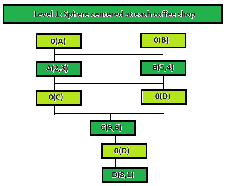
ball tree algorithm

When searching for the nearest coffee shop, the Ball Tree algorithm eliminates entire spheres that are farther away than the current best candidate. It provides a different way of efficiently pruning the search space compared to the KD-Tree.

Suppose you start searching for the nearest coffee shop from your location. The KD-Tree might guide you by asking whether the coffee shop is to the left or right of a certain street, efficiently narrowing down your search. On the other hand, the Ball Tree might eliminate entire neighborhoods if they are farther away than the current best option, providing a different way to prune the search space.

In both cases, these algorithms help you efficiently navigate the city’s space to find the nearest coffee shop, demonstrating the power of spatial indexing for real-world applications.

Key Concepts of Ball Tree Algorithm

Here are the key concepts related to the Ball Tree algorithm:

1. Hypersphere:

• In the context of the Ball Tree algorithm, a hypersphere is a generalization of a sphere to higher dimensions. It is defined by a center point and a radius, representing all points in the space that are a certain distance (radius) away from the center.

2. Node:

• Each node in the Ball Tree represents a hypersphere that encloses a subset of the data points. The center and radius of the hypersphere are determined based on the points within that node.

3. Root Node:

• The topmost node in the Ball Tree, representing the entire dataset. The root node’s hypersphere encompasses all the data points.

4. Leaf Node:

• A leaf node is a node in the Ball Tree that doesn’t have any child nodes. Each leaf node corresponds to a subset of the data points, and the hypersphere it represents encloses those points.

5. Splitting Criteria:

• The Ball Tree recursively splits the dataset into subsets based on a splitting criterion. This criterion is often chosen to maximize the spread of the hyperspheres or optimize some distance metric.

6. Partitioning Dimension:

• In each level of the tree, the algorithm chooses a specific dimension along which to partition the data. This decision is based on the splitting criterion and aims to create hyperspheres that efficiently enclose data points.

7. Hierarchical Structure:

• The Ball Tree forms a hierarchical structure with parent-child relationships. Each node in the tree has two child nodes, forming a binary tree. The structure allows for efficient pruning of the search space during nearest neighbor queries.

8. Distance Metric:

• The choice of distance metric is crucial in defining the hyperspheres and determining the nearest neighbors. Common distance metrics include Euclidean distance, Manhattan distance, and Minkowski distance.

9. Nearest Neighbor Search:

• The primary purpose of the Ball Tree is to facilitate efficient nearest neighbor searches. During a search, the algorithm navigates the tree, eliminating entire hyperspheres that cannot contain a closer neighbor than the current best candidate. This pruning process significantly reduces the search space.

10. Balancing:

• Balancing is a crucial aspect of constructing an effective Ball Tree. It ensures that the hyperspheres are evenly distributed throughout the tree, preventing skewed structures that might hinder the efficiency of nearest neighbor searches.

11. Construction Algorithm:

• The construction algorithm for a Ball Tree involves recursively partitioning the dataset and assigning hyperspheres to each node. The choice of splitting dimension and the balancing strategy impact the overall performance of the tree.

Ball Trees are particularly useful in applications where nearest neighbor searches need to be performed efficiently in high-dimensional spaces, such as clustering, classification, and anomaly detection in machine learning. The algorithm provides a flexible and adaptive way to organize and search multidimensional data.

Implementation of Ball Tree Algorithm

Python

from sklearn.neighbors import BallTree
import numpy as np

# Sample 2D dataset
data = np.array([[2, 3], [5, 4], [9, 6], [8, 1]])

# Constructing Ball Tree
ball_tree = BallTree(data)

# Query point
query_point = np.array([[3, 5]])

# Finding the nearest neighbor
distances, indices = ball_tree.query(query_point, k=1)

print("Dataset:")
print(data)

print("\nBall Tree Structure:")
print(ball_tree)

print("\nQuery Point:")
print(query_point)

print("\nNearest Neighbor:")
print("Index:", indices[0])
print("Point:", data[indices[0]])
print("Distance:", distances[0])

Output:

Dataset:
[[2 3]
 [5 4]
 [9 6]
 [8 1]]
Ball Tree Structure:
<sklearn.neighbors._ball_tree.BallTree object at 0x0000020568CA7D00>
Query Point:
[[3 5]]
Nearest Neighbor:
Index: [0]
Point: [[2 3]]
Distance: [2.23606798]

This code illustrates how to use the scikit-learn BallTree algorithm. ‘Data’, the 2D dataset, is first created. This dataset is used to build the BallTree. Once ‘query_point’ is defined, a BallTree query is performed to determine the query point’s closest neighbor (k=1). The original dataset, the BallTree structure, the query point, and information about the closest neighbor, including its index, coordinates, and distance from the query point, are all included in the output.

Difference between Ball Tree Algorithm and KD Tree Algorithm

The key difference in Ball Tree Algorithm and KD Tree Algorithm are:

Feature	Ball Tree	KD-Tree
Splitting Strategy	Ball Tree divides the data into hyperspheres, which are multidimensional spheres.	KD-Tree divides the data using axis-aligned hyperplanes, essentially creating rectangular partitions.
Space Partitioning	Ball Tree organizes data in hierarchical hyperspheres.	KD-Tree organizes data using hierarchical axis-aligned rectangles.
Tree Structure	Ball Tree is non-binary, meaning each node can have multiple children.	KD-Tree is binary, with each node having exactly two children.
Dimensionality	Ball Tree is effective for low to moderate dimensions.	KD-Tree is effective for low to high dimensions.
Nearest Neighbor Search	Ball Tree is generally faster for sparse high-dimensional data.	KD-Tree is efficient for low to moderate dimensions in nearest neighbor searches.
Tree Construction	Ball Tree construction is slower due to complex geometric computations involved	KD-Tree construction is generally faster due to its simpler structure.
Balancing	Ball Tree is naturally balanced.	KD-Tree may require balancing strategies to maintain a balanced tree.
Memory Usage	Ball Tree typically has higher memory usage.	KD-Tree generally has lower memory usage.
Implementation Complexity	Ball Tree implementation is more complex due to its non-binary structure.	KD-Tree implementation is simpler due to its binary tree structure.
Query Time Complexity	Both have logarithmic query time complexity in average cases.	Both have logarithmic query time complexity in average cases.
Applications	Ball Tree is often used for sparse, high-dimensional data.	KD-Tree is commonly used for low to moderate dimensions in various applications.
Library Implementations	Ball Tree is implemented in libraries like Scikit-learn and SciPy.	KD-Tree is implemented in libraries such as Scikit-learn, SciPy, and various others.

Frequently Asked Questions

Q1: What is the main difference between Ball Tree and KD-Tree algorithms?

The main difference lies in their splitting strategies and tree structures. Ball Tree divides data into hyperspheres using a non-binary structure, while KD-Tree employs axis-aligned hyperplanes with a binary tree structure.

Q2: In what scenarios is the Ball Tree algorithm more suitable?

Ball Tree is often preferred for sparse, high-dimensional data where hypersphere partitioning is effective. It excels in scenarios with low to moderate dimensions and is used in applications like nearest neighbor searches for such data.

Q3: When should I consider using the KD-Tree algorithm?

KD-Tree is a good choice for low to high-dimensional data and is particularly efficient in applications where the data can be effectively partitioned using axis-aligned hyperplanes. It is commonly used for moderate-dimensional data in various applications.

Q4: How does the construction time differ between Ball Tree and KD-Tree?

Ball Tree construction is generally slower due to complex geometric computations, whereas KD-Tree construction is faster due to its simpler binary structure.

Q5: Are there any memory usage differences between the two algorithms?

Yes, Ball Tree typically has higher memory usage compared to KD-Tree, making KD-Tree more memory-efficient.

Q6: Do both algorithms have logarithmic query time complexity?

Yes, both Ball Tree and KD-Tree algorithms exhibit logarithmic query time complexity in average cases, making them efficient for search operations.