LSTM – Derivation of Back propagation through time
Last Updated :
27 Dec, 2021
LSTM (Long short term Memory ) is a type of RNN(Recurrent neural network), which is a famous deep learning algorithm that is well suited for making predictions and classification with a flavour of the time. In this article, we will derive the algorithm backpropagation through time and find the gradient value for all the weights at a particular timestamp.
As the name suggests backpropagation through time is similar to backpropagation in DNN(deep neural network) but due to the dependency of time in RNN and LSTM, we will have to apply the chain rule with time dependency.
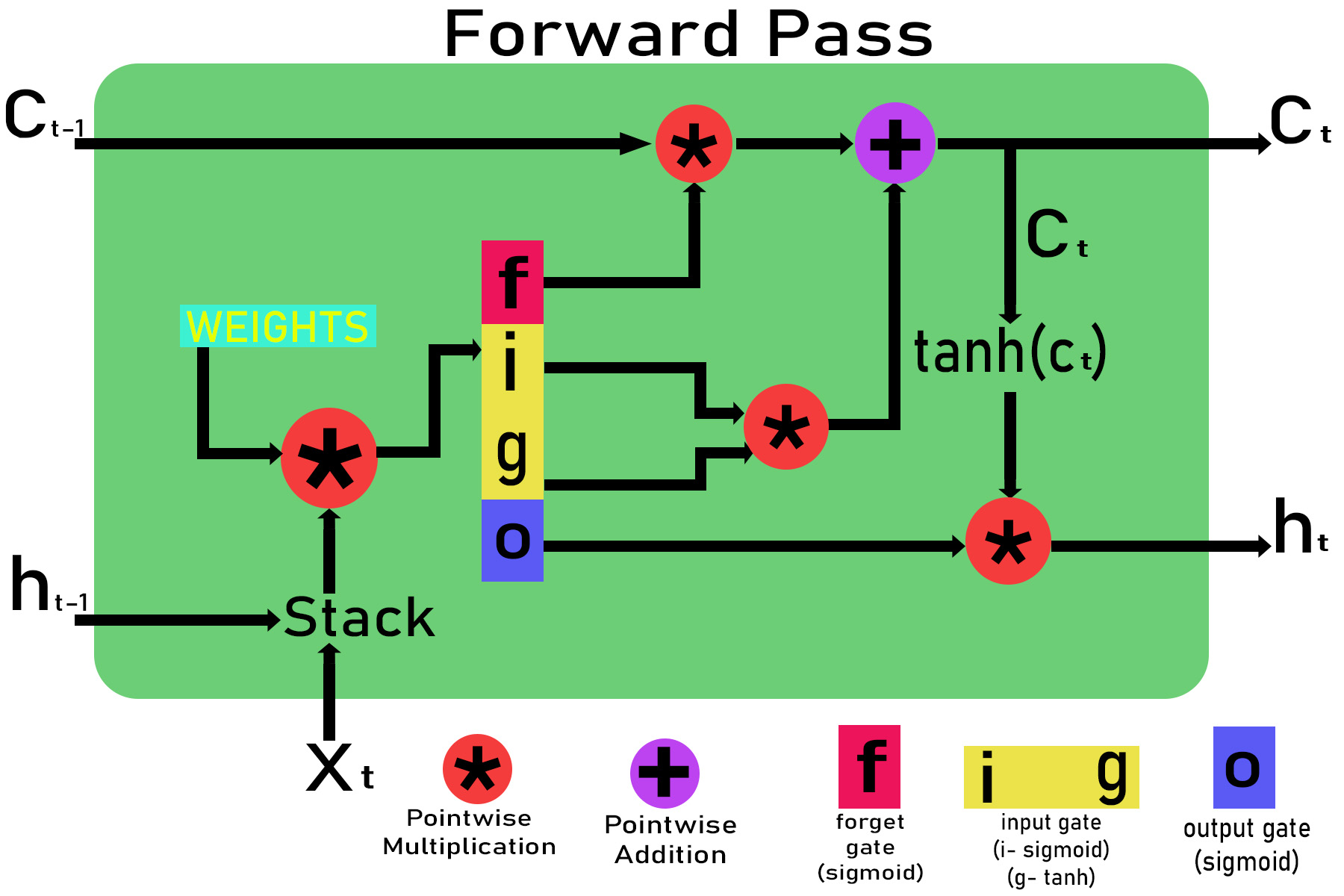
Let the input at time t in the LSTM cell be xt, the cell state from time t-1 and t be ct-1 and ct and the output for time t-1 and t be ht-1 and ht . The initial value of ct and ht at t = 0 will be zero.
Step 1 : Initialization of the weights .
Weights for different gates are :
Input gate : wxi, wxg, bi, whj, wg , bg

Forget gate : wxf, bf, whf

Output gate : wxo, bo, who
Step 2 : Passing through different gates .
Inputs: xt and ht-i , ct-1  are given to the LSTM cell
      Passing through input gate:

          Zg = wxg *x + whg * ht-1 + bg
          g = tanh(Zg)
          Zj = wxi * x + whi * ht-1 + bi
          i =  sigmoid(Zi)

          Input_gate_out = g*i

      Passing through forget gate:

          Zf = wxf * x + whf *ht-1 + bf
          f = sigmoid(Zf)

      Forget_gate_out = f

      Passing through the output gate:

      Zo  = wxo*x +  who * ht-1 + bo
      o = sigmoid(zO)

      Out_gate_out = o
Step 3 : Calculating the output ht and current cell state ct.
  Calculating the current cell state ct :
          ct = (ct-1 * forget_gate_out) + input_gate_out

Calculating the output gate ht:
          ht=out_gate_out * tanh(ct)
Step 4 : Calculating the gradient through back propagation through time at time stamp t using the chain rule.
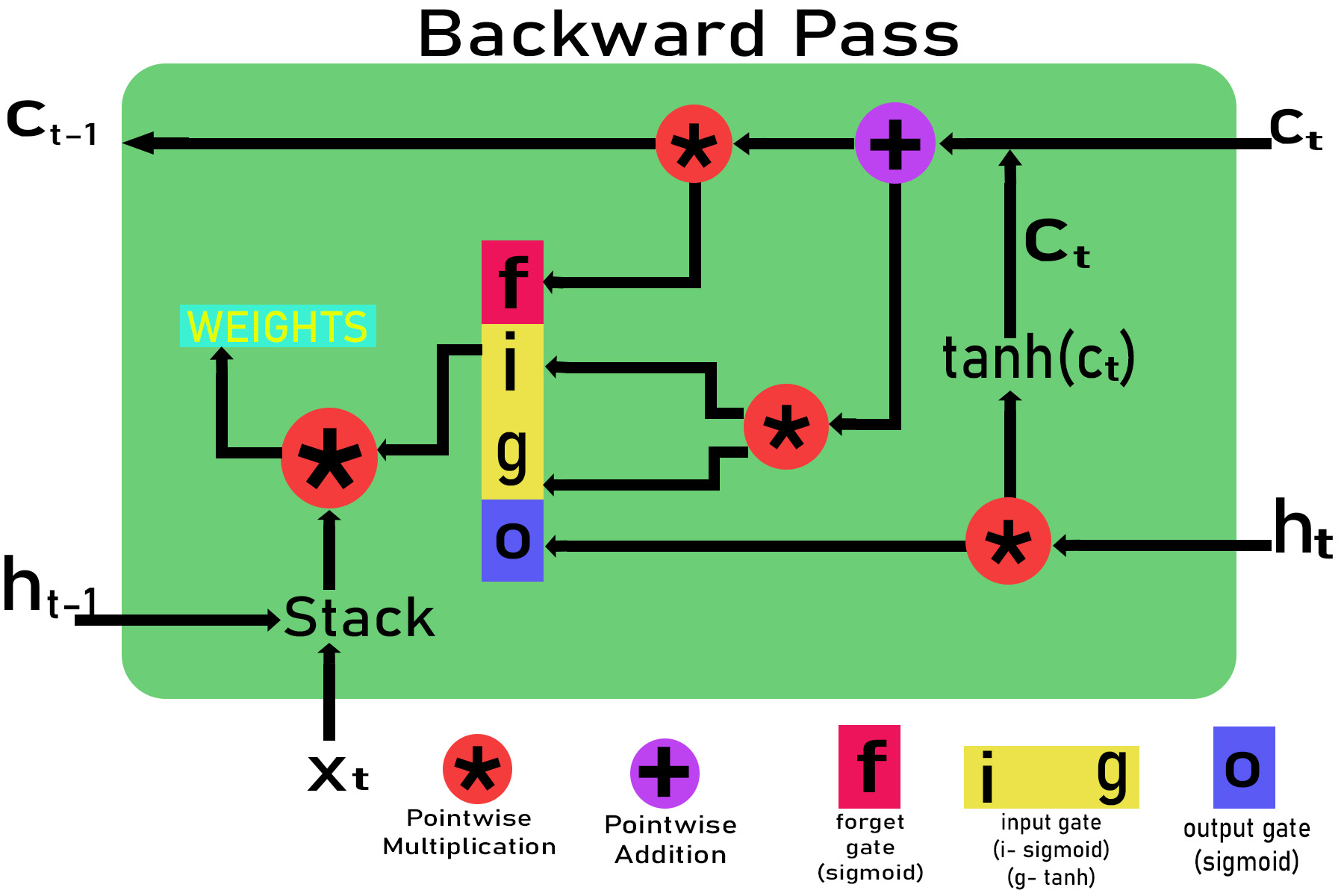
  Let the gradient pass down by the above cell be:
      E_delta  = dE/dht

      If we are using MSE (mean square error)for error then,
      E_delta=(y-h(x))
      Here y is the original value and h(x) is the predicted value.

  Gradient with respect to output gate

             dE/do = (dE/dht ) * (dht /do) = E_delta * ( dht / do)
                dE/do =  E_delta * tanh(ct)

  Gradient with respect to ct
      dE/dct = (dE / dht )*(dht /dct)= E_delta *(dht /dct)
                dE/dct  =   E_delta   * o * (1-tanh2 (ct))

  Gradient with respect to input gate dE/di, dE/dg

      dE/di = (dE/di ) * (dct / di)
             dE/di =  E_delta   * o * (1-tanh2 (ct)) * g
      Similarly,
      dE/dg =  E_delta   * o * (1-tanh2 (ct)) * i

  Gradient with respect to forget gate

          dE/df =  E_delta   * (dE/dct ) * (dct / dt) t
          dE/df =  E_delta   * o * (1-tanh2 (ct)) *  ct-1

  Gradient with respect to ct-1

          dE/dct =  E_delta   * (dE/dct ) * (dct / dct-1)
          dE/dct =  E_delta   * o * (1-tanh2 (ct)) * f

  Gradient with respect to output gate weights:

    dE/dwxo   =  dE/do *(do/dwxo) = E_delta * tanh(ct) * sigmoid(zo) * (1-sigmoid(zo) * xt
    dE/dwho   =  dE/do *(do/dwho) = E_delta * tanh(ct) * sigmoid(zo) * (1-sigmoid(zo) * ht-1
    dE/dbo   =  dE/do *(do/dbo) = E_delta * tanh(ct) * sigmoid(zo) * (1-sigmoid(zo)

   Gradient with respect to forget gate weights:

    dE/dwxf  =  dE/df *(df/dwxf) = E_delta * o * (1-tanh2 (ct)) * ct-1 * sigmoid(zf) * (1-sigmoid(zf) * xt
    dE/dwhf =  dE/df *(df/dwhf) = E_delta * o * (1-tanh2 (ct)) *  ct-1 * sigmoid(zf) * (1-sigmoid(zf) * ht-1
    dE/dbo  =  dE/df *(df/dbo) = E_delta * o * (1-tanh2 (ct)) *  ct-1 * sigmoid(zf) * (1-sigmoid(zf)

   Gradient with respect to input gate weights:

    dE/dwxi  =  dE/di *(di/dwxi) = E_delta * o * (1-tanh2 (ct)) * g * sigmoid(zi) * (1-sigmoid(zi) * xt
    dE/dwhi =  dE/di *(di/dwhi) = E_delta * o * (1-tanh2 (ct)) * g * sigmoid(zi) * (1-sigmoid(zi) * ht-1
    dE/dbi  =  dE/di *(di/dbi) = E_delta * o * (1-tanh2 (ct)) * g *  sigmoid(zi) * (1-sigmoid(zi)

    dE/dwxg  =  dE/dg *(dg/dwxg) = E_delta * o * (1-tanh2 (ct)) * i * (1?tanh2(zg))*xt
    dE/dwhg  =  dE/dg *(dg/dwhg) = E_delta * o * (1-tanh2 (ct)) * i * (1?tanh2(zg))*ht-1
    dE/dbg  =  dE/dg *(dg/dbg)  = E_delta * o * (1-tanh2 (ct)) * i * (1?tanh2(zg))
Finally the gradients associated with the weights are,
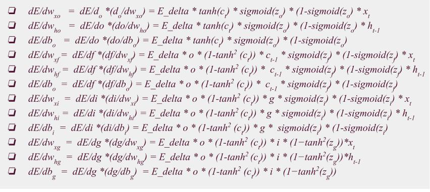
Using all gradient, we can easily update the weights associated with input gate, output gate, and forget gate
Share your thoughts in the comments
Please Login to comment...