Affinity Propagation in ML | To find the number of clusters
Last Updated :
14 May, 2019
Affinity Propagation creates clusters by sending messages between data points until convergence. Unlike clustering algorithms such as k-means or k-medoids, affinity propagation does not require the number of clusters to be determined or estimated before running the algorithm, for this purpose the two important parameters are the preference, which controls how many exemplars (or prototypes) are used, and the damping factor which damps the responsibility and availability of messages to avoid numerical oscillations when updating these messages.
A dataset is described using a small number of exemplars, ‘exemplars’ are members of the input set that are representative of clusters. The messages sent between pairs represent the suitability for one sample to be the exemplar of the other, which is updated in response to the values from other pairs. This updating happens iteratively until convergence, at that point the final exemplars are chosen, and hence we obtain the final clustering.
Algorithm for Affinity Propagation:
Input: Given a dataset D = {d1, d2, d3, …..dn}
s is a NxN matrix such that s(i, j) represents the similarity between di and dj. The negative squared distance of two data points was used as s i.e. for points xi and xj, s(i, j)= -||xi-xj||2 .
The diagonal of s i.e. s(i, i) is particularly important, as it represents the input preference, meaning how likely a particular input is to become an exemplar. When it is set to the same value for all inputs, it controls how many classes the algorithm produces. A value close to the minimum possible similarity produces fewer classes, while a value close to or larger than the maximum possible similarity, produces many classes. It is typically initialized to the median similarity of all pairs of inputs.
The algorithm proceeds by alternating two message passing steps, to update two matrices:
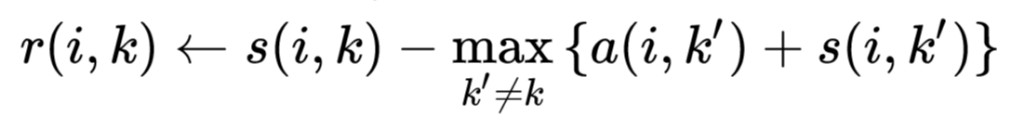
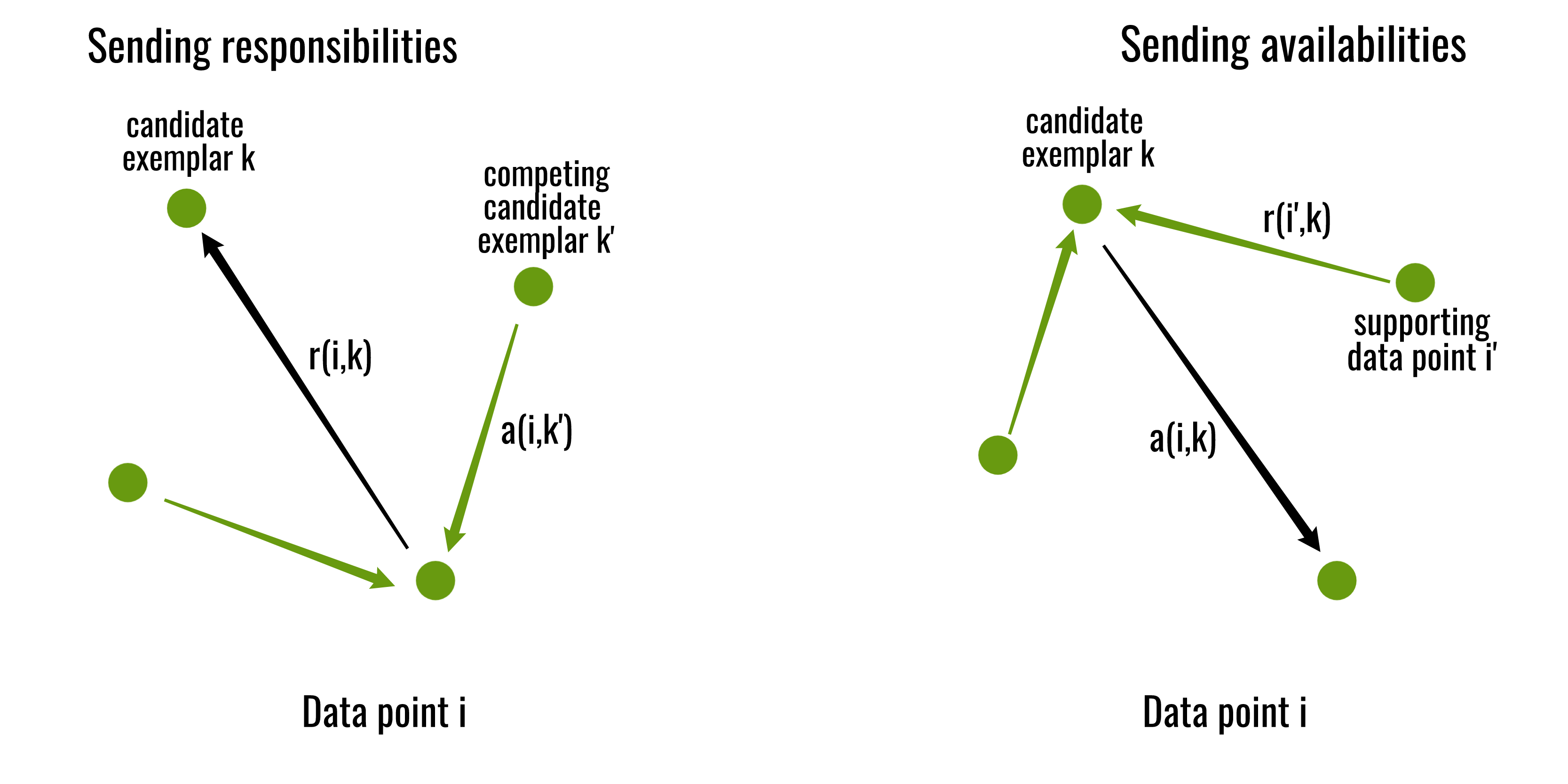
- The “responsibility” matrix R has values r(i, k) that quantify how well-suited xk is to serve as the exemplar for xi, relative to other candidate exemplars for xi.
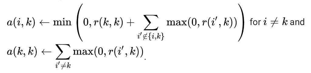
- The “availability” matrix A contains values a(i, k) that represent how “appropriate” it would be for xi to pick xk as its exemplar, taking into account other points’ preference for xk as an exemplar.
Both matrices are initialized to all zeroes. The algorithm then performs the following updates iteratively:
- First, responsibility updates are sent around
- Then, availability is updated per
The iterations are performed until either the cluster boundaries remain unchanged over a number of iterations, or after some predetermined number of iterations. The exemplars are extracted from the final matrices as those whose ‘responsibility + availability’ for themselves is positive (i.e. (r(i, i) + a(i, i)) > 0).
Below is the Python implementation of the Affinity Propagation clustering using scikit-learn library:
from sklearn.cluster import AffinityPropagation
from sklearn import metrics
from sklearn.datasets.samples_generator import make_blobs
centers = [[1, 1], [-1, -1], [1, -1], [-1, -1]]
X, labels_true = make_blobs(n_samples = 400, centers = centers,
cluster_std = 0.5, random_state = 0)
af = AffinityPropagation(preference =-50).fit(X)
cluster_centers_indices = af.cluster_centers_indices_
labels = af.labels_
n_clusters_ = len(cluster_centers_indices)
|
import matplotlib.pyplot as plt
from itertools import cycle
plt.close('all')
plt.figure(1)
plt.clf()
colors = cycle('bgrcmykbgrcmykbgrcmykbgrcmyk')
for k, col in zip(range(n_clusters_), colors):
class_members = labels == k
cluster_center = X[cluster_centers_indices[k]]
plt.plot(X[class_members, 0], X[class_members, 1], col + '.')
plt.plot(cluster_center[0], cluster_center[1], 'o',
markerfacecolor = col, markeredgecolor ='k',
markersize = 14)
for x in X[class_members]:
plt.plot([cluster_center[0], x[0]],
[cluster_center[1], x[1]], col)
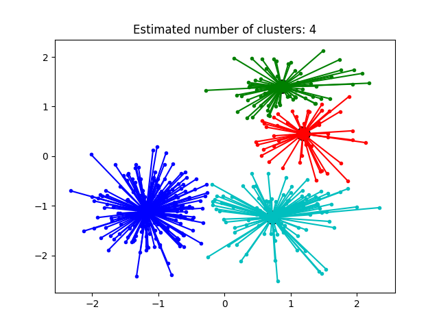
plt.title('Estimated number of clusters: % d' % n_clusters_)
plt.show()
|
Output:
Like Article
Suggest improvement
Share your thoughts in the comments
Please Login to comment...