Train and Test Neural Networks Using R

Training and testing neural networks using R is a fundamental aspect of machine learning and deep learning. In this comprehensive guide, we will explore the theory and practical steps involved in building, training, and evaluating neural networks in R Programming Language. Neural networks are a class of machine learning models inspired by the human brain, and they have achieved remarkable success in a wide range of applications, including image recognition, natural language processing, and predictive modelling.

What is a Neural Network?

A neural network, also known as an artificial neural network (ANN), is a computational model that is loosely inspired by the structure and function of the human brain. It consists of interconnected nodes, or artificial neurons, organized in layers. These layers are typically categorized into three types:

• Input Layer: This layer receives the raw data or features, and each neuron represents an input feature.
• Hidden Layers: These layers perform complex transformations on the input data. A neural network can have multiple hidden layers, and each layer can contain multiple neurons.
• Output Layer: The final layer provides the network’s predictions or outputs. The number of neurons in the output layer depends on the specific problem, such as binary classification, multi-class classification, or regression.

How Neural Networks Work

Neural networks work by passing information from one layer to the next through weighted connections. Each connection has an associated weight, and each neuron computes a weighted sum of its inputs, applies an activation function, and passes the result to the next layer. The activation function introduces non-linearity into the network, allowing it to model complex relationships.

The training process involves adjusting the weights to minimize the difference between the network’s predictions and the actual target values. This is achieved through optimization algorithms like gradient descent, which iteratively update the weights to reduce the loss or error of the model.

Practical Implementation in R

Now, let’s delve into the practical steps for training and testing neural networks using R.

Data Preparation

• Before you can start building a neural network, you need to prepare your data. Data preparation includes the following tasks.
• Data Loading: Import your dataset into R. You can use functions like read.csv for CSV files or readRDS for RDS files.
• Data Exploration: Understand your data by exploring its features, distributions, and statistical properties. This will help you identify any missing values or outliers.
• Data Splitting: Divide your data into two sets: a training set and a testing set. A common split ratio is 70-30 or 80-20 for training and testing, respectively.

R

# Load necessary libraries
library(tensorflow)
library(keras)

# Generate a synthetic dataset
set.seed(42)

# Number of samples
n_samples <- 1000

# Simulated features
X <- matrix(runif(n_samples * 4), ncol = 4)

# Simulated labels (binary classification)
y <- as.integer(X[, 1] + X[, 2] + X[, 3] > 1.5)

Model Construction

In R, you can use the keras library, which provides a high-level interface for building and training neural networks. Here’s how to construct a neural network model using keras.

Data Preprocessing: Prepare your data for training by performing tasks like feature scaling (e.g., standardization or normalization), one-hot encoding for categorical variables, and handling missing values.

R

# Data preprocessing (optional but recommended)
X_train <- scale(X_train)
X_test <- scale(X_test)

Model Compilation

After constructing the neural network, you need to compile it by specifying the loss function, optimizer, and evaluation metrics. The choice of these components depends on your specific problem type (e.g., classification or regression).

R

# Create a neural network model
model <- keras_model_sequential()
model %>%
  layer_dense(units = 64, activation = 'relu', input_shape = 4) %>%
  layer_dense(units = 32, activation = 'relu') %>%
  layer_dense(units = 1, activation = 'sigmoid')

Model Training

Now, you are ready to train your neural network using the training data. Training involves iteratively updating the model’s weights to minimize the specified loss function.

R

# Compile the model
model %>%
  compile(
    loss = 'binary_crossentropy',
    optimizer = optimizer_adam(lr = 0.001),
    metrics = c('accuracy')
  )

# Train the model
history <- model %>%
  fit(
    X_train, y_train,
    epochs = 50,
    batch_size = 32,
    validation_data = list(X_test, y_test)
  )

Output:

Epoch 1/50
22/22 [==============================] - 9s 195ms/step - loss: 0.6452 - accuracy: 0.6700 - val_loss: 0.5492 - val_accuracy: 0.8700
Epoch 2/50
22/22 [==============================] - 1s 33ms/step - loss: 0.4794 - accuracy: 0.9043 - val_loss: 0.3927 - val_accuracy: 0.9300
Epoch 3/50
22/22 [==============================] - 1s 48ms/step - loss: 0.3396 - accuracy: 0.9371 - val_loss: 0.2688 - val_accuracy: 0.9533
Epoch 4/50
22/22 [==============================] - 1s 43ms/step - loss: 0.2327 - accuracy: 0.9771 - val_loss: 0.1867 - val_accuracy: 0.9733
Epoch 5/50
22/22 [==============================] - 1s 39ms/step - loss: 0.1658 - accuracy: 0.9829 - val_loss: 0.1386 - val_accuracy: 0.9733
Epoch 6/50
22/22 [==============================] - 1s 44ms/step - loss: 0.1270 - accuracy: 0.9829 - val_loss: 0.1100 - val_accuracy: 0.9767
Epoch 7/50
22/22 [==============================] - 1s 51ms/step - loss: 0.1021 - accuracy: 0.9900 - val_loss: 0.0913 - val_accuracy: 0.9767
Epoch 8/50
22/22 [==============================] - 1s 41ms/step - loss: 0.0862 - accuracy: 0.9900 - val_loss: 0.0795 - val_accuracy: 0.9767
Epoch 9/50
22/22 [==============================] - 1s 41ms/step - loss: 0.0750 - accuracy: 0.9943 - val_loss: 0.0715 - val_accuracy: 0.9767
Epoch 10/50
22/22 [==============================] - 1s 39ms/step - loss: 0.0671 - accuracy: 0.9886 - val_loss: 0.0642 - val_accuracy: 0.9767
Epoch 11/50
22/22 [==============================] - 1s 42ms/step - loss: 0.0596 - accuracy: 0.9971 - val_loss: 0.0610 - val_accuracy: 0.9767
Epoch 12/50
22/22 [==============================] - 1s 35ms/step - loss: 0.0542 - accuracy: 0.9943 - val_loss: 0.0563 - val_accuracy: 0.9767
Epoch 13/50
22/22 [==============================] - 1s 34ms/step - loss: 0.0500 - accuracy: 0.9957 - val_loss: 0.0533 - val_accuracy: 0.9767
Epoch 14/50
22/22 [==============================] - 1s 43ms/step - loss: 0.0466 - accuracy: 0.9943 - val_loss: 0.0511 - val_accuracy: 0.9767
Epoch 15/50
22/22 [==============================] - 1s 39ms/step - loss: 0.0443 - accuracy: 0.9929 - val_loss: 0.0491 - val_accuracy: 0.9767
Epoch 16/50
22/22 [==============================] - 1s 39ms/step - loss: 0.0415 - accuracy: 0.9943 - val_loss: 0.0470 - val_accuracy: 0.9767
Epoch 17/50
22/22 [==============================] - 1s 39ms/step - loss: 0.0389 - accuracy: 0.9943 - val_loss: 0.0451 - val_accuracy: 0.9767
Epoch 18/50
22/22 [==============================] - 1s 36ms/step - loss: 0.0375 - accuracy: 0.9957 - val_loss: 0.0440 - val_accuracy: 0.9767
Epoch 19/50
22/22 [==============================] - 1s 35ms/step - loss: 0.0353 - accuracy: 0.9943 - val_loss: 0.0445 - val_accuracy: 0.9767
Epoch 20/50
22/22 [==============================] - 1s 40ms/step - loss: 0.0341 - accuracy: 0.9943 - val_loss: 0.0429 - val_accuracy: 0.9767
Epoch 21/50
22/22 [==============================] - 1s 47ms/step - loss: 0.0317 - accuracy: 1.0000 - val_loss: 0.0416 - val_accuracy: 0.9767
Epoch 22/50
22/22 [==============================] - 1s 44ms/step - loss: 0.0311 - accuracy: 0.9971 - val_loss: 0.0406 - val_accuracy: 0.9767
Epoch 23/50
22/22 [==============================] - 1s 37ms/step - loss: 0.0290 - accuracy: 0.9971 - val_loss: 0.0389 - val_accuracy: 0.9767
Epoch 24/50
22/22 [==============================] - 1s 39ms/step - loss: 0.0289 - accuracy: 0.9971 - val_loss: 0.0422 - val_accuracy: 0.9733
Epoch 25/50
22/22 [==============================] - 1s 33ms/step - loss: 0.0274 - accuracy: 0.9971 - val_loss: 0.0362 - val_accuracy: 0.9767
Epoch 26/50
22/22 [==============================] - 1s 40ms/step - loss: 0.0270 - accuracy: 0.9971 - val_loss: 0.0395 - val_accuracy: 0.9767
Epoch 27/50
22/22 [==============================] - 1s 46ms/step - loss: 0.0256 - accuracy: 0.9971 - val_loss: 0.0387 - val_accuracy: 0.9767
Epoch 28/50
22/22 [==============================] - 1s 37ms/step - loss: 0.0261 - accuracy: 0.9957 - val_loss: 0.0388 - val_accuracy: 0.9767
Epoch 29/50
22/22 [==============================] - 1s 39ms/step - loss: 0.0241 - accuracy: 0.9971 - val_loss: 0.0362 - val_accuracy: 0.9767
Epoch 30/50
22/22 [==============================] - 1s 36ms/step - loss: 0.0252 - accuracy: 0.9943 - val_loss: 0.0365 - val_accuracy: 0.9767
Epoch 31/50
22/22 [==============================] - 1s 33ms/step - loss: 0.0243 - accuracy: 0.9929 - val_loss: 0.0417 - val_accuracy: 0.9733
Epoch 32/50
22/22 [==============================] - 1s 39ms/step - loss: 0.0227 - accuracy: 0.9957 - val_loss: 0.0385 - val_accuracy: 0.9767
Epoch 33/50
22/22 [==============================] - 1s 40ms/step - loss: 0.0216 - accuracy: 0.9986 - val_loss: 0.0386 - val_accuracy: 0.9767
Epoch 34/50
22/22 [==============================] - 1s 38ms/step - loss: 0.0209 - accuracy: 0.9986 - val_loss: 0.0391 - val_accuracy: 0.9733
Epoch 35/50
22/22 [==============================] - 1s 36ms/step - loss: 0.0196 - accuracy: 0.9971 - val_loss: 0.0358 - val_accuracy: 0.9767
Epoch 36/50
22/22 [==============================] - 1s 34ms/step - loss: 0.0191 - accuracy: 1.0000 - val_loss: 0.0373 - val_accuracy: 0.9767
Epoch 37/50
22/22 [==============================] - 1s 42ms/step - loss: 0.0190 - accuracy: 0.9986 - val_loss: 0.0367 - val_accuracy: 0.9767
Epoch 38/50
22/22 [==============================] - 1s 38ms/step - loss: 0.0184 - accuracy: 0.9957 - val_loss: 0.0380 - val_accuracy: 0.9767
Epoch 39/50
22/22 [==============================] - 1s 42ms/step - loss: 0.0180 - accuracy: 1.0000 - val_loss: 0.0354 - val_accuracy: 0.9767
Epoch 40/50
22/22 [==============================] - 1s 36ms/step - loss: 0.0173 - accuracy: 1.0000 - val_loss: 0.0344 - val_accuracy: 0.9767
Epoch 41/50
22/22 [==============================] - 1s 34ms/step - loss: 0.0178 - accuracy: 0.9943 - val_loss: 0.0375 - val_accuracy: 0.9767
Epoch 42/50
22/22 [==============================] - 1s 38ms/step - loss: 0.0178 - accuracy: 0.9971 - val_loss: 0.0392 - val_accuracy: 0.9767
Epoch 43/50
22/22 [==============================] - 1s 40ms/step - loss: 0.0168 - accuracy: 0.9971 - val_loss: 0.0410 - val_accuracy: 0.9733
Epoch 44/50
22/22 [==============================] - 1s 39ms/step - loss: 0.0180 - accuracy: 0.9971 - val_loss: 0.0393 - val_accuracy: 0.9767
Epoch 45/50
22/22 [==============================] - 1s 36ms/step - loss: 0.0165 - accuracy: 0.9971 - val_loss: 0.0334 - val_accuracy: 0.9767
Epoch 46/50
22/22 [==============================] - 1s 33ms/step - loss: 0.0153 - accuracy: 1.0000 - val_loss: 0.0375 - val_accuracy: 0.9767
Epoch 47/50
22/22 [==============================] - 1s 41ms/step - loss: 0.0151 - accuracy: 0.9971 - val_loss: 0.0373 - val_accuracy: 0.9767
Epoch 48/50
22/22 [==============================] - 1s 40ms/step - loss: 0.0142 - accuracy: 0.9986 - val_loss: 0.0330 - val_accuracy: 0.9767
Epoch 49/50
22/22 [==============================] - 1s 52ms/step - loss: 0.0140 - accuracy: 1.0000 - val_loss: 0.0379 - val_accuracy: 0.9767
Epoch 50/50
22/22 [==============================] - 1s 39ms/step - loss: 0.0141 - accuracy: 0.9986 - val_loss: 0.0339 - val_accuracy: 0.9767

Train and Test Neural Networks Using R

A random seed is set to ensure reproducibility.

• n_samples is defined as the number of data points (1,000 in this case).
• Synthetic features X are generated as a 1,000×4 matrix with random values.
• Simulated labels y are created for binary classification based on a condition involving the first three columns of X.
• The dataset is divided into training and testing sets using random sampling. In this example, 70% of the data is used for training, and 30% is reserved for testing.
• A neural network model is created using the Keras library. This model is a sequential model, which means you can add layers one after the other. In this case, a feedforward neural network is built with two hidden layers. The architecture is as follows.
  • Input layer: It has 4 units (one for each feature) and uses the ReLU activation function.
  • First hidden layer: It has 64 units and uses the ReLU activation function.
  • Second hidden layer: It has 32 units and uses the ReLU activation function.
  • Output layer: It has 1 unit for binary classification and uses the sigmoid activation function.
• After constructing the model, it is compiled with specific configuration. The compilation involves specifying the loss function, the optimizer, and the evaluation metric. In this case, the binary cross-entropy loss is chosen for binary classification, the Adam optimizer with a learning rate of 0.001 is used, and accuracy is chosen as the evaluation metric.

The model is trained on the training data. The training process involves iterating over the dataset for a specified number of epochs (50 in this example) and updating the model’s weights to minimize the loss. The training data is divided into mini-batches of size 32 for each iteration. The validation data is provided to monitor the model’s performance during training.

Model Evaluation

After training, it’s crucial to evaluate your model’s performance on a separate testing dataset. This allows you to assess how well your model generalizes to unseen data. Common evaluation metrics include accuracy, precision, recall, F1-score, and more, depending on your problem.

Now we Create a complex dataset and performing all the operations on it in a single response is a substantial task. Instead, I’ll provide you with a simplified example that you can follow. In practice, complex datasets can vary widely, and the specific dataset you work with will depend on your application. Here’s a simplified example using a synthetic dataset for binary classification.

R

# Evaluate the model
evaluation <- model %>% evaluate(X_test, y_test)
print(evaluation)

Output:

      loss   accuracy 
0.03387477 0.97666669 

The evaluation results indicate that your trained neural network achieved an accuracy of approximately 97.67% on the test data. This means that it correctly classified 97.67% of the test samples, which is an excellent result. The loss value of approximately 0.03387477 indicates how well the model is fitting the data, with lower values being better.

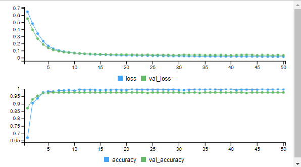
Plot the model

By using plot function we can plot the model.

R

plot(history)

Output:

Train and Test Neural Networks Using R