Positive and Negative Trend Arrows in Excel
Last Updated :
27 May, 2021
A Positive Trend is an up arrow that indicates an upward trend and a Negative Trend is a down arrow that indicates a downward trend. In this article, we will look into how we can create Positive And Negative Trends in Excel.
To do so follow the below steps:
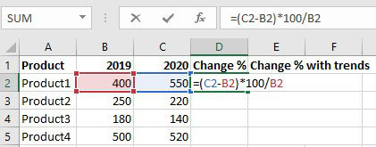
Step 1: First format your data.

Step 2: Calculate the change % between two year.
- Firstly, we will write =(C2-B2)*100/B2 in the first cell of Change%.
- Then, we will get the Change% for Product1.

- Drag the Change% of Product1 to get remaining Products Change%.

To add Up and Down Arrows:
Step 1: Select an empty cell.
Step 2: Then, click to the Insert tab on the Ribbon. In the Symbols group, click Symbol.

Step 3: In the Symbol box scroll down and select the up arrow and then click Insert to add on the selected cell.

Step 4: To add down arrow follow the above step 1 and 2 then in the Symbol box scroll down and select down arrow and then click Insert to add on the selected cell.

Now, the up and down arrows both are added in the selected cells which are C8 for the up arrow and D8 for the down arrow.
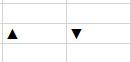
Arrows
Now, we will use these two cells to fill the column with Change% with trends.
Step 5: In the first cell of Change% with trends we will write =D2&IF(D2>0,C8,D8).

- Then, we will get the Change% with trends for Product1.

- Drag the Change% with trends of Product1 to get remaining Products Change% with trends.

Share your thoughts in the comments
Please Login to comment...