How to Rotate Pie Charts in Excel?
Last Updated :
09 May, 2021
A Pie Chart is a circular statistical graphic, which is divided into slices to illustrate numerical proportion.In this article, we’ll see how we can create and rotate pie charts.
How to make Pie Charts in Excel ?
Follow the below steps to create a pie chart in Excel:
Step 1: Formatting data for pie charts
Just we have to make sure that categories and associated values are each on separate lines.
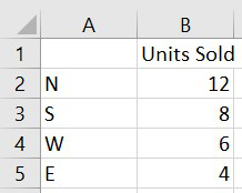
Here, we’ll use the number of units sold for a range of products.
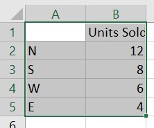
Step 2: Converting the data into pie chart
First, highlight the data which we want in the pie chart.
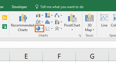
Then click to the Insert tab on the Ribbon. In the Charts group, click Insert Pie or Doughnut Chart
In the resulting menu, click 2D Pie.
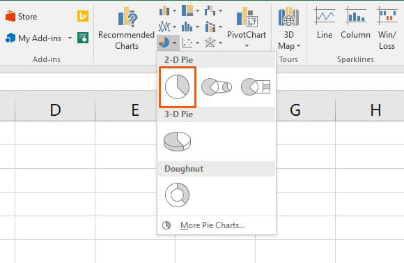
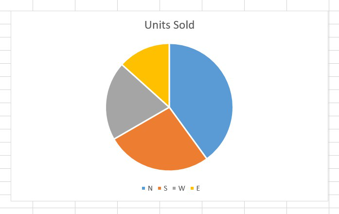
Once we have clicked that, our Pie chart will appear.
How to rotate the Pie Charts in Excel?
Now, we will see how to rotate the Pie Chart.
Step 1: Double-click the pie chart to enable Format Data Series… panel on the right of Excel spreadsheet, or we can right-click it and choose Format Data Series in the menu.
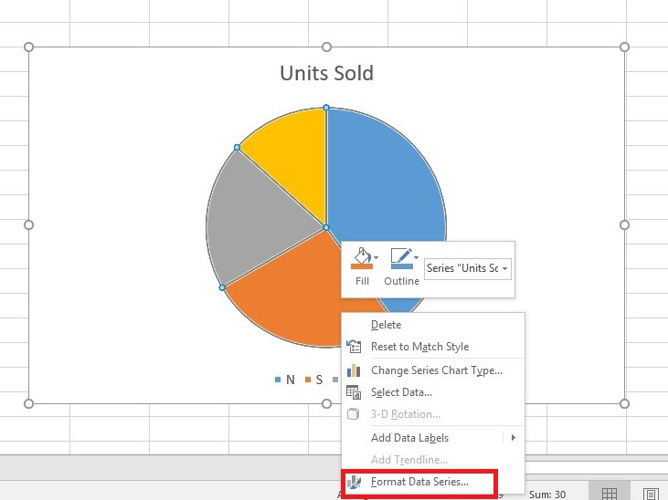
The Format Data Series panel will show on the right of the page.
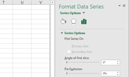
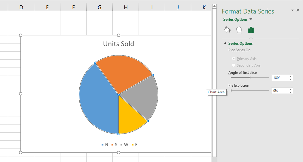
Step 2: Switch to Series Options (the icon of histogram) and we can adjust the Angle of first slice here. Change the value in the textbox, the pie chart will rotate accordingly.
Share your thoughts in the comments
Please Login to comment...