PCA and SVM Pipeline in Python

Principal Component Analysis (PCA) and Support Vector Machines (SVM) are powerful techniques used in machine learning for dimensionality reduction and classification, respectively. Combining them into a pipeline can enhance the performance of the overall system, especially when dealing with high-dimensional data. The aim of the article is demonstrate how we can utilize PCA and SVM in single pipeline in Python.

What is a support vector machine?

Support Vector Machine is used for classification and regression problems. At first it was used for only classification problems. It works by finding the best hyperplane that separates the different classes. The hyperplane is selected by maximizing the margin between the classes.

What is PCA?

Principal Component Analysis is a technique used for dimensionality reduction in machine learning. It is useful for converting larger datasets into smaller datasets with maintaining all the patterns. It helps reduce the features in the data while preserving the maximum amount of information.

Why use Pipeline?

A machine learning pipeline is like an assembly line where many processes are are connected sequentially, such as preparing data, training the data, etc. So, it becomes easier to work with from start to end.

Even we can do our all our task from training to testing without the pipeline, so what is the real benefit of using pipeline? There are many reasons to use pipeline, let’s discuss few of them:

1. When using pipeline, same preprocessing steps can be applied to both training and testing data without writing different code for both of them.
2. It encapsulates the entire work into single object.
3. It is most useful when label encoding has to be done for both training and testing.
4. It reduces the code length as when we want to train for multiple times we can use that pipeline.

Implementation of PCA and SVM in a Pipeline

Importing Required Libraries

Python3

import pandas as pd
import seaborn as sns
from sklearn.svm import SVC
import matplotlib.pyplot as plt
from sklearn.decomposition import PCA
from sklearn.pipeline import Pipeline
from sklearn.metrics import confusion_matrix
from sklearn.model_selection import train_test_split
from sklearn.metrics import classification_report

Loading the dataset and Preprocessing

Python3

# Load the dataset
from sklearn import datasets
cancer = datasets.load_breast_cancer()

Convert loaded data into DataFrame

Python3

# converting into dataframe
df = pd.DataFrame(data=cancer.data, columns=cancer.feature_names)

# adding target column to the df
df['target'] = cancer.target

Understanding the data

Python3

# Shape of the dataset
print("Shape of the dataset:", df.shape)

# unique values in the target columns
print(df.target.unique())

# Printing 5 randome sample from the dataset
df.sample(5)

Output:

Shape of the dataset: (569, 31)
[0 1]
mean radius    mean texture    mean perimeter    mean area    mean smoothness    mean compactness    mean concavity    mean concave points    mean symmetry    mean fractal dimension    ...    worst texture    worst perimeter    worst area    worst smoothness    worst compactness    worst concavity    worst concave points    worst symmetry    worst fractal dimension    target
86    14.48    21.46    94.25    648.2    0.09444    0.09947    0.12040    0.04938    0.2075    0.05636    ...    29.25    108.40    808.9    0.1306    0.1976    0.3349    0.12250    0.3020    0.06846    0
554    12.88    28.92    82.50    514.3    0.08123    0.05824    0.06195    0.02343    0.1566    0.05708    ...    35.74    88.84    595.7    0.1227    0.1620    0.2439    0.06493    0.2372    0.07242    1
221    13.56    13.90    88.59    561.3    0.10510    0.11920    0.07860    0.04451    0.1962    0.06303    ...    17.13    101.10    686.6    0.1376    0.2698    0.2577    0.09090    0.3065    0.08177    1
510    11.74    14.69    76.31    426.0    0.08099    0.09661    0.06726    0.02639    0.1499    0.06758    ...    17.60    81.25    473.8    0.1073    0.2793    0.2690    0.10560    0.2604    0.09879    1
118    15.78    22.91    105.70    782.6    0.11550    0.17520    0.21330    0.09479    0.2096    0.07331    ...    30.50    130.30    1272.0    0.1855    0.4925    0.7356    0.20340    0.3274    0.12520    0
5 rows × 31 columns

So as you can see the data consists of 5 rows and 31 columns, and in target column there are two classes 0 and 1, so it is a classification problem, so we will use Support Vector Machine, and as you can see there are 30 features so here we can apply principal component analysis for reducing the features.

Splitting Data in training and testing

Python3

# X contains all columns except target column
X = df.drop(['target'], axis=1)
print("Shape of X:", X.shape)

# y contains target column
y = df['target']
print("Shape of y:", y.shape)

# Splitting data into training and testing
X_train, X_test, y_train, y_test = train_test_split(X, y, test_size=0.2, random_state=10)
print("Shape of X_train:", X_train.shape)
print("Shape of X_test:", X_test.shape)
print("Shape of y_train", y_train.shape)
print("Shape of y_test", y_test.shape)

Output:

Shape of X: (569, 30)
Shape of y: (569,)
Shape of X_train: (455, 30)
Shape of X_test: (114, 30)
Shape of y_train (455,)
Shape of y_test (114,)

Our data is spillted into 80% training and 20% testing and we have provided random state so if we rerun the code then also same spilliting will be done.

Creating Pipeline

Python3

# Pipeline with PCA and SVM
clf = Pipeline([
    ("pca",PCA(n_components=0.7)),
    ("svm",SVC(C=10,kernel='rbf')),
])

#Training the data
clf.fit(X_train,y_train)

Output:

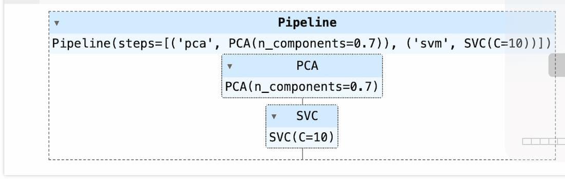
SVM with PCA

So, as you can see with pipeline, we don’t have to use any fit_transform instead it will be taken care by pipeline, additionally if there are more preprocessing steps you can include them in the pipeline and train it.

Using PCA and SVM in a pipeline streamlines the modeling process by combining preprocessing (dimensionality reduction) and modeling (SVM classification) into a single workflow. This simplifies code maintenance and facilitates reproducibility.

Prediction using the model

Python3

# score of testing data
print("Score is:",clf.score(X_test,y_test))

# precision recall f1-score support report
y_pred = clf.predict(X_test)
report = classification_report(y_test, y_pred)
print("Classificaion Report")
print(report)

Output:

Score is: 0.8859649122807017
Classificaion Report
              precision    recall  f1-score   support

           0       0.91      0.74      0.82        39
           1       0.88      0.96      0.92        75

    accuracy                           0.89       114
   macro avg       0.89      0.85      0.87       114
weighted avg       0.89      0.89      0.88       114

Confusion Matrix

Python3

# confusion matrix
cm = confusion_matrix(y_test,y_pred)
print(cm)

# using seaborn
sns.heatmap(cm,annot=True)
plt.ylabel("Truth")
plt.xlabel("Predicted")

Output:

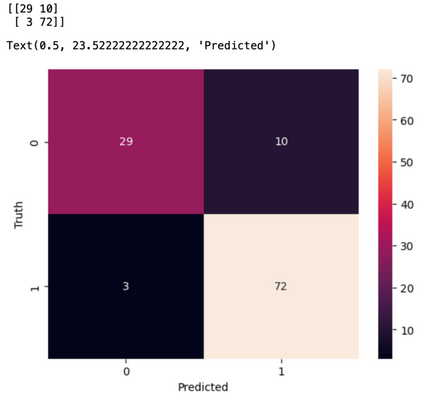
When we use Principal Component Analysis and Support Vector Machine together in pipeline, it becomes a smooth process for preparing our data before building our model. It is useful when data is complex and large and want to achieve a good accuracy on our model.