Visualizing Support Vector Machines (SVM) using Python

Support Vector Machines (SVMs) are powerful supervised learning models used for classification and regression tasks. A key factor behind their popularity is their ability to handle both linear and non-linear data effectively. In this article, we will explore visualizing SVMs using Python and popular libraries like scikit-learn and Matplotlib.

Support Vector Machine (SVMs)

Support Vector Machines work by finding the optimal hyperplane that best separates the classes in the feature space. The hyperplane is chosen to maximize the margin, which is the distance between the hyperplane and the nearest data points from each class, known as support vectors. This hyperplane is determined by solving an optimization problem, which aims to minimize the classification error while maximizing the margin.

SVMs can be used for both linear and non-linear classification tasks through the use of different kernel functions like linear, polynomial, radial basis function (RBF), and sigmoid kernels. These kernels allow SVMs to handle non-linear decision boundaries by mapping the original feature space into a higher-dimensional space where the classes become separable.

Visualizing Linear SVMs

Let’s start by visualizing a simple linear SVM using Iris dataset. We will generate the data and train the SVM model using Scikit-Learn. Then, we’ll plot the decision boundary and support vectors to understand how the model separates the classes.

Importing Necessary Libraries and load the Dataset

This dataset contains measurements of sepal and petal dimensions for three species of iris flowers. Here, only the first two features (sepal length and sepal width) are retained for visualization purposes.

Python3

import numpy as np
import matplotlib.pyplot as plt
from sklearn import datasets
from sklearn.svm import SVC
iris = datasets.load_iris()
X = iris.data[:, :2]  # Only first two features for visualization
y = iris.target

Training SVM with Linear Kernel

An SVM model with a linear kernel is trained on the Iris dataset. A linear kernel is suitable for linearly separable data, aiming to find the best hyperplane that separates different classes.

Python3

# Train SVM with linear kernel
clf_linear = SVC(kernel='linear')
clf_linear.fit(X, y)

Creating Meshgrid for Decision Boundary

A meshgrid is created to cover the feature space. This allows for the generation of points for visualization purposes. The decision boundaries of the SVM models will be plotted on this meshgrid.

Python3

# Create a mesh to plot decision boundaries
h = 0.02  # step size in the mesh
x_min, x_max = X[:, 0].min() - 1, X[:, 0].max() + 1
y_min, y_max = X[:, 1].min() - 1, X[:, 1].max() + 1
xx, yy = np.meshgrid(np.arange(x_min, x_max, h),
                     np.arange(y_min, y_max, h))

Plotting Decision Boundary of Linear SVM

The decision boundary of the SVM with a linear kernel is plotted. This is achieved by predicting the class labels for all points on the meshgrid using the predict method. The decision boundary is then visualized using filled contour plots (plt.contourf) and original data points are overlaid on the plot for reference.

Python3

# Plot decision boundary of Linear SVM
Z_linear = clf_linear.predict(np.c_[xx.ravel(), yy.ravel()])
Z_linear = Z_linear.reshape(xx.shape)
plt.contourf(xx, yy, Z_linear, cmap=plt.cm.Paired, alpha=0.8)
plt.scatter(X[:, 0], X[:, 1], c=y, cmap=plt.cm.Paired)
plt.title('Linear SVM')
plt.xlabel('Sepal Length')
plt.ylabel('Sepal Width')
plt.xlim(xx.min(), xx.max())
plt.ylim(yy.min(), yy.max())
plt.show()

Output:

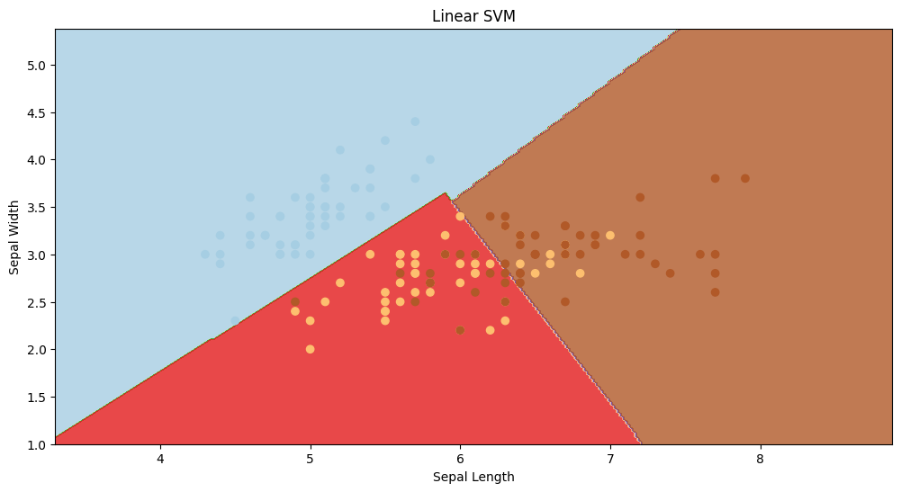
linear SVM visualisation

In the above visualization, linear SVM has classified the data points in a linear way. Even though the accuracy is not that great, we can clearly see that the red section has a ton of misclassified datapoints, but that’s where non-linear svm will come into picture.

Visualizing Non-linear SVMs

SVMs can also handle non-linear decision boundaries by using kernel functions. Let’s visualize a non-linear SVM using the same Iris dataset with a polynomial kernel.

Understanding the Impact of Gamma in RBF Kernels

Before visualizing non-linear SVMs, let’s explore the influence of the gamma parameter in the RBF kernel.

The gamma parameter significantly impacts the RBF kernel’s behavior in SVMs. It essentially determines the influence of individual data points on the decision boundary.

• A lower gamma value results in a wider influence of each data point, leading to a smoother decision boundary.
• Conversely, a higher gamma value narrows the influence of data points, creating a more complex and potentially overfitted decision boundary.

Defining Gamma Values

A list named gamma_values is defined, containing different values of the gamma hyperparameters, controlling the influence of a single training example.

Python3

import numpy as np
import matplotlib.pyplot as plt
from sklearn import datasets
from sklearn.svm import SVC
iris = datasets.load_iris()
X = iris.data[:, :2]  # Only first two features for visualization
y = iris.target

gamma_values = [0.1, 1, 10, 50, 100, 200]

Plotting Decision Boundaries for Each Gamma Value

1. A figure is created with a size of 20×10 inches to accommodate subplots for each gamma value. The code iterates over each gamma value in the gamma_values list. For each gamma value, an SVM model with an RBF kernel is trained using the specified gamma value.
2. Inside the loop, a meshgrid is created to cover the feature space, allowing for the generation of points for visualization purposes. The meshgrid is defined with a step size of 0.02.
3. For each gamma value, the decision boundary of the SVM with an RBF kernel is plotted. This is achieved by predicting the class labels for all points on the meshgrid using the predict method.
4. The decision boundary is then visualized using filled contour plots (plt.contourf). Original data points are overlaid on the plot for reference, with colors corresponding to their respective class labels.

Python3

# Plot decision boundaries for each gamma value
plt.figure(figsize=(20, 10))
for i, gamma in enumerate(gamma_values, 1):
    # Train SVM with RBF kernel
    clf_rbf = SVC(kernel='rbf', gamma=gamma)
    clf_rbf.fit(X, y)

    # Create a mesh to plot decision boundaries
    h = 0.02  # step size in the mesh
    x_min, x_max = X[:, 0].min() - 1, X[:, 0].max() + 1
    y_min, y_max = X[:, 1].min() - 1, X[:, 1].max() + 1
    xx, yy = np.meshgrid(np.arange(x_min, x_max, h),
                         np.arange(y_min, y_max, h))

    # Plot decision boundary
    plt.subplot(2, 3, i)
    Z_rbf = clf_rbf.predict(np.c_[xx.ravel(), yy.ravel()])
    Z_rbf = Z_rbf.reshape(xx.shape)
    plt.contourf(xx, yy, Z_rbf, cmap=plt.cm.Paired, alpha=0.8)
    plt.scatter(X[:, 0], X[:, 1], c=y, cmap=plt.cm.Paired)
    plt.title(f'RBF SVM (Gamma={gamma})')
    plt.xlabel('Sepal Length')
    plt.ylabel('Sepal Width')
    plt.xlim(xx.min(), xx.max())
    plt.ylim(yy.min(), yy.max())

plt.tight_layout()
plt.show()

Output:

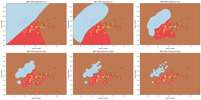
Non linear SVM visualisation with different gamma values

In the above visualization, clearly gamma values impacts a lot on the accuracy and complexity of the model.

• We chose 6 different gamma values and due to that we have 6 different visualization, higher the gamma value, higher the accuracy, that’s why in the visualization where the gamma value is 200, our model has classified the data points almost perfectly.
• But when it comes to the model where we have chosen gamma value as 50, its alsmot very similar to the result of linear SVM and the accuracy is not that high too.

Conclusion

In conclusion, Support Vector Machines (SVMs) are powerful models for both linear and non-linear classification tasks. Visualizing SVMs, especially with different kernels and hyperparameters, provides valuable insights into their behavior and performance.