Multioutput Regression in Machine Learning

In machine learning we often encounter regression, these problems involve predicting a continuous target variable, such as house prices, or temperature. However, in many real-world scenarios, we need to predict not only single but many variables together, this is where we use multi-output regression.

In this article, we will understand the topic of multi-output regression and how to implement it using Scikit-learn in Python.

Multi-output Regression

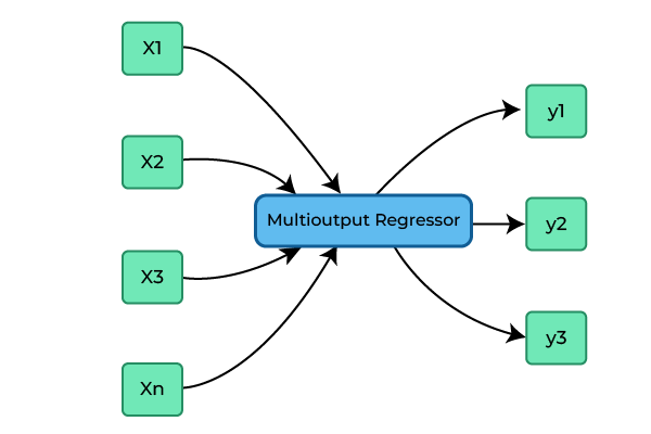
We know in simple regression we predict a single output variable but where the goal is to predict multiple target variables instead of just one we use Multi-output regression. Multi-output regression is mostly used for addressing complex real-world problems. This approach is particularly useful when variables are interrelated or when it is more efficient to make joint predictions as the prediction of one variable can affect the prediction of other variables, we’ll understand this thing in the subtopic of chained regression.

It can be represented as follows:

where:

• y1, y2, …, ym are the output variables
• x1, x2, …, xn are the input variables
• f is the regression function

Multioutput regression

Multi-output Regression using Scikit-learn

Let’s start understanding the multi-output regression using Scikit-learn with an example using the UCI Energy efficiency dataset.

The dataset we’ll explore is the Energy Efficiency dataset from the UCI Machine Learning Repository. This dataset contains eight input variables and two output variables, making it suitable for multi-output regression. The variables are following:

Features (Independent variables)

• X1 Relative Compactness
• X2 Surface Area
• X3 Wall Area
• X4 Roof Area
• X5 Overall Height
• X6 Orientation
• X7 Glazing Area
• X8 Glazing Area Distribution

Outputs (Dependent variables)

• y1 Heating Load
• y2 Cooling Load

Step 1: Downloading and unzipping the dataset

Python

import urllib.request
from zipfile import ZipFile

# Downloading data
urllib.request.urlretrieve(
    "https://archive.ics.uci.edu/static/public/242/energy+efficiency.zip", "data.zip")

# Unzipping data.zip
with ZipFile("data.zip", 'r') as zipref:
    zipref.extractall('.')

We are downloading the dataset using the urllib.request library by specifying the URL of the ZIP file to be downloaded and the we save it as “data.zip” in the current directory. Next, we use the ZipFile module from the zipfile library to extract the contents of the ZIP file into the current directory, after extracting we will have an excel file “ENB2012_data.xlsx”.

Step 2: Reading dataset using Pandas

Now, we are using the pandas library to read this excel file and store its contents in a dataframe named ‘df’.

Once the data is loaded into df, we display the first 5 rows of the dataframe using the head() method.

Python

import pandas as pd
df = pd.read_excel('ENB2012_data.xlsx')
df.head()

Output:

     X1     X2     X3      X4   X5  X6   X7  X8     Y1     Y2
0  0.98  514.5  294.0  110.25  7.0   2  0.0   0  15.55  21.33
1  0.98  514.5  294.0  110.25  7.0   3  0.0   0  15.55  21.33
2  0.98  514.5  294.0  110.25  7.0   4  0.0   0  15.55  21.33
3  0.98  514.5  294.0  110.25  7.0   5  0.0   0  15.55  21.33
4  0.90  563.5  318.5  122.50  7.0   2  0.0   0  20.84  28.28

Step 3: Exploratory data analysis (EDA)

(i) Visualize the correlations between different features

Using Seaborn and Matplotlib we are visualizing the correlations,

• df.corr() method calculates the correlation between the features.
• sns.heatmap() function generates a heatmap of the correlation matrix passed to it, here we are setting cbar=False and annot=True, to remove color bar and annotate the heatmap cells with the correlation values.

Python

# Finding correlation between features and plotting them
import seaborn as sns
import matplotlib.pyplot as plt
plt.figure(figsize = (8,5))
sns.heatmap(df.corr(), cbar = False, annot = True, fmt=".1f")

Output:

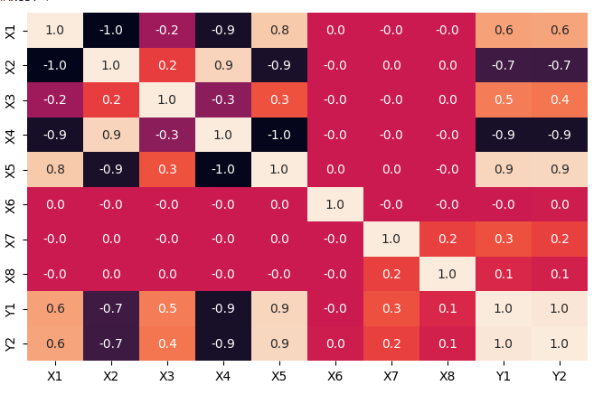
Correlation between different features in the dataset

Analysis:

• There is a strong correlation of X1, X3, X5, and X7 with both Y1 and Y2, indicating their influence on the output variables.
• X1, X5, and X2, X4 exhibit significant correlations with one another, suggesting interdependencies among these input variables.
• The dependent variables Y1 and Y2 demonstrate a notable correlation of 0.98, signifying a strong relationship between them.

(ii) Plotting histograms to visualize data distribution

For each feature, a histogram is plotted with a kernel density estimation (KDE) curve, providing insights into the data distribution.

• plt.subplots(nrows, ncols): Creates a grid of subplots with the specified number of rows and columns.
• sns.histplot(): Generates a histogram plot with an optional KDE curve to visualize the distribution of data for a given feature.

Python

import matplotlib.pyplot as plt

# Define the number of rows and columns you want
n_rows=2
n_cols=4

# Create the subplots
fig, axes = plt.subplots(nrows=n_rows, ncols=n_cols)
fig.set_size_inches(10, 5)
for i, column in enumerate(df.iloc[:, :-2].columns):
    sns.histplot(df[column], ax=axes[i//n_cols, i % n_cols], kde=True)
plt.tight_layout()

Output:

(iv) Finding unique values in each feature to understand the variance:

Python

for col in X_train.columns:
    print(f"{col} : ", X_train[f'{col}'].unique())

Output

X1 :  [0.82 0.64 0.86 0.9  0.66 0.79 0.62 0.76 0.69 0.74 0.98 0.71]
X2 :  [612.5 784.  588.  563.5 759.5 637.  808.5 661.5 735.  686.  514.5 710.5]
X3 :  [318.5 343.  294.  367.5 416.5 245.  269.5]
X4 :  [147.   220.5  122.5  110.25]
X5 :  [7.  3.5]
X6 :  [2 4 5 3]
X7 :  [0.1  0.4  0.25 0.  ]
X8 :  [1 2 4 3 5 0]

Analysis:

Based on the histograms, it’s evident that

• X3, X4, X5, X6, X7, and X8 exhibit a predominantly categorical nature.
• X1 and X2, while displaying some variation, lean more towards being continuous features.

The feature suggests a tendency towards categorical characteristics in the dataset.

(v) Regression plot of each feature wrt. Y1

Here we are exploring the relationships between each feature in the dataframe and the ‘Y1’ output variable.

• sns.regplot() is used here to create scatter plots with regression lines for each feature against ‘Y1’. The scatter points are marked in green, and the regression lines are depicted in red.
• scatter_kws and line_kws: These parameters allow customization of the appearance of the scatter points and the regression line in the plot.

Python

# Create the subplots
fig, axes = plt.subplots(nrows=n_rows, ncols=n_cols)
fig.set_size_inches(10, 5)
for i, column in enumerate(df.iloc[:,:-2].columns):
    sns.regplot(x = df[column], y = df['Y1'],ax=axes[i//n_cols,i%n_cols], scatter_kws={"color": "green"}, line_kws={"color": "red"})
plt.tight_layout()

Output:

Analysis

Most features are not linearly separable with respect to dependent variable Y1.

(vi) Regression plot of each feature wrt. Y2

The code remains unchanged, we have only substituted the y-axis variable, with ‘Y2’ in place of ‘Y1.’

Python

# Create the subplots
fig, axes = plt.subplots(nrows=n_rows, ncols=n_cols)
fig.set_size_inches(10, 5)
for i, column in enumerate(df.iloc[:,:-2].columns):
    sns.regplot(x = df[column], y = df['Y2'],ax=axes[i//n_cols,i%n_cols], scatter_kws={"color": "black" , 'cmap':'jet'}, line_kws={"color": "red"})
plt.tight_layout()

Output:

Analysis

Same as ‘Y1,’ the analysis reveals that the relationships between the features and ‘Y2’ are not linearly separable, indicating the absence of straightforward linear patterns in the data.

Step 4: Utility function to print result metrics

Here I’m creating a utility functions showResults() and printPredictions() to print the output regression metrics and predicted values.

Python

from sklearn.metrics import mean_squared_error
from sklearn.metrics import r2_score
from sklearn.metrics import mean_absolute_error

def printPredictions(y_true,y_pred, count):
  print(f"Predictions: ")
  print(y_true.assign(
      Y1_pred = y_pred[:,0],
      Y2_pred = y_pred[:,1]
  ).head(count).to_markdown(index = False))

def showResults(y_true, y_pred, count = 5):
  print("R2 score: ",r2_score(y_true,y_pred))
  print("Mean squared error: ",mean_squared_error(y_true,y_pred))
  print("Mean absolute error: ",mean_absolute_error(y_true,y_pred))
  printPredictions(y_true,y_pred, count)

• printPredictions(y_true, y_pred, count): This function prints a summary of predictions. It takes true and predicted values an arguments and after combining it prints them in a tabular format.
  
• showResults(y_true, y_pred, count=5): It calculates the key regression metrics,
  • R-squared (R2) score.
  • Mean squared error (MSE)
  • Mean absolute error (MAE).

Step 5: Splitting data into train and test data

This code uses scikit-learn’s train_test_split function to split a dataset into training and testing sets.
The data is divided such that 80% is used for training, and 20% is reserved for testing. The random_state parameter ensures reproducibility.

Python

from sklearn.model_selection import train_test_split
X_train,X_test,y_train,y_test = train_test_split(df.iloc[:,:-2], df.iloc[:,-2:], test_size = 0.2, random_state = 42)
print(X_train.shape,X_test.shape)
print(y_train.shape, y_test.shape)

Output:

((614, 8), (154, 8))
((614, 2), (154, 2))

Step 6: Creating multi-output regression model

The multi-output regression using Scikit-learn can be done in three ways:

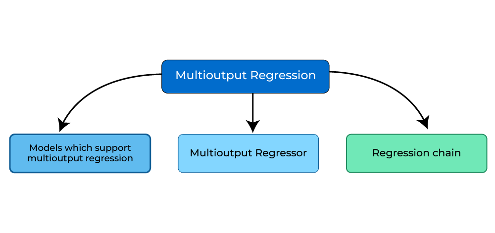
1. Models which support Multi-output regression

There are several models that are capable of performing multi-output regression, here are few of them:

• Linear Regression
• Random Forest Regressor
• Extra Trees Regressor
• K-Neighbors Regressor

(i) Linear regression

The simplest of all regressions which assumes a linear relationship between input features and target variables.

Python

from sklearn.linear_model import LinearRegression

linear = LinearRegression()
linear.fit(X_train,y_train)
showResults(y_test,linear.predict(X_test))

Output:

R2 score:  0.9028145634342284
Mean squared error:  9.51221811381318
Mean absolute error:  2.187258158162318
Predictions: 
|    Y1 |    Y2 |   Y1_pred |   Y2_pred |
|------:|------:|----------:|----------:|
| 16.47 | 16.9  |   18.8418 |   19.7585 |
| 13.17 | 16.39 |   14.0391 |   16.7736 |
| 32.82 | 32.78 |   31.3253 |   32.0241 |
| 41.32 | 46.23 |   35.9226 |   36.7056 |
| 16.69 | 19.76 |   15.3271 |   17.2817 |

(ii) Random forest regressor

An ensemble learning technique that combines multiple decision trees to provide an accurate predictions for regression tasks.

Python

from sklearn.ensemble import RandomForestRegressor
rdf = RandomForestRegressor()
rdf.fit(X_train,y_train)
showResults(y_test,rdf.predict(X_test))

Output:

R2 score:  0.9791808278921088
Mean squared error:  1.9422728968506515
Mean absolute error:  0.75378538961039
Predictions: 
|    Y1 |    Y2 |   Y1_pred |   Y2_pred |
|------:|------:|----------:|----------:|
| 16.47 | 16.9  |   15.5453 |   17.1487 |
| 13.17 | 16.39 |   13.1251 |   16.1184 |
| 32.82 | 32.78 |   32.6253 |   33.2548 |
| 41.32 | 46.23 |   41.8913 |   42.9433 |
| 16.69 | 19.76 |   16.8311 |   19.8748 |

(iii) Extra trees regressor

Random forest sub-samples the input data with replacement, whereas Extra Trees use the whole original sample and also adds randomness in the tree-building process by choosing random split instead of an optimum one.

Python

from sklearn.ensemble import ExtraTreesRegressor
extra_reg = ExtraTreesRegressor()
extra_reg.fit(X_train,y_train)
showResults(y_test,extra_reg.predict(X_test))

Output:

R2 score:  0.982457926794601
Mean squared error:  1.6381520869480493
Mean absolute error:  0.6900980519480521
Predictions: 
|    Y1 |    Y2 |   Y1_pred |   Y2_pred |
|------:|------:|----------:|----------:|
| 16.47 | 16.9  |   15.3672 |   17.1868 |
| 13.17 | 16.39 |   13.1397 |   16.1522 |
| 32.82 | 32.78 |   32.8389 |   32.9537 |
| 41.32 | 46.23 |   41.9232 |   43.1254 |
| 16.69 | 19.76 |   16.7657 |   20.0407 |

(iv) K-neighbours regressor

This model estimates target values based on the proximity of neighbors, making it adaptable and effective for multi-output regression, especially when local patterns matter among the features.

Python

from sklearn.neighbors import KNeighborsRegressor
knn = KNeighborsRegressor()
knn.fit(X_train,y_train)
showResults(y_test,knn.predict(X_test))

Output:

R2 score:  0.9552345708141144
Mean squared error:  4.417399493506494
Mean absolute error:  1.5228636363636365
Predictions: 
|    Y1 |    Y2 |   Y1_pred |   Y2_pred |
|------:|------:|----------:|----------:|
| 16.47 | 16.9  |    14.408 |    15.384 |
| 13.17 | 16.39 |    13.65  |    16.602 |
| 32.82 | 32.78 |    30.262 |    30.852 |
| 41.32 | 46.23 |    40.496 |    44.61  |
| 16.69 | 19.76 |    16.946 |    20.164 |

Analysis

Given that the data is primarily categorical in nature, the R2 score for Linear Regression is the lowest at 0.902, while the Extra-Trees Regressor achieves the highest R2 score of 0.98. It’s possible to enhance the R2 score further by doing hyperparamter tuning.

2. Using MultiOutputRegressor()

Here we train a separate regressor for each target variable. It’s a straightforward method to expand the capabilities of regressors that aren’t inherently designed for multi-target regression tasks.

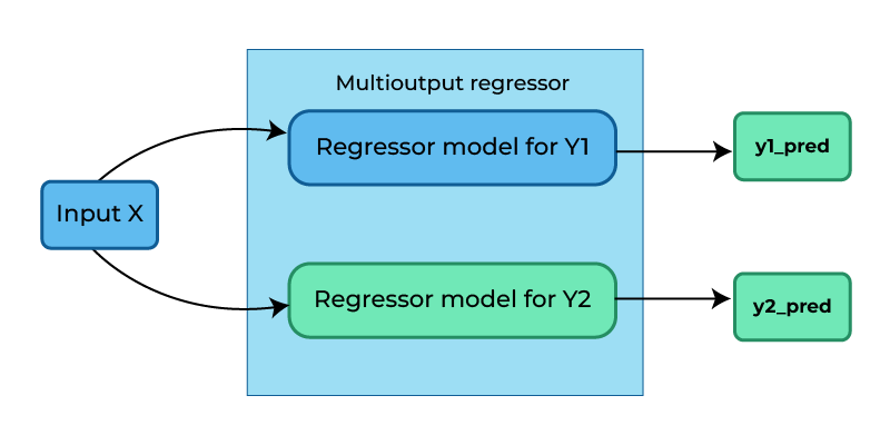
We are implementing a multi-output regression model using the Support Vector Regressor (SVR) from scikit-learn. Here we pass SVR which is originally designed for single-output regression tasks to MultiOutputRegressor, which acts like a wrapper over SVR, this extends SVR to handle the multi-output regression effectively.

Python

from sklearn.multioutput import MultiOutputRegressor
from sklearn.svm import SVR

svm_multi = MultiOutputRegressor(SVR(kernel="rbf", C=100, gamma=0.1, epsilon=0.1))
svm_multi.fit(X_train,y_train)
showResults(y_test,svm_multi.predict(X_test))

Output:

R2 score:  0.9876712414729131
Mean squared error:  1.1737865734622686
Mean absolute error:  0.64545622613329
Predictions: 
|    Y1 |    Y2 |   Y1_pred |   Y2_pred |
|------:|------:|----------:|----------:|
| 16.47 | 16.9  |   15.4987 |   16.426  |
| 13.17 | 16.39 |   12.9448 |   16.4907 |
| 32.82 | 32.78 |   32.2836 |   32.5228 |
| 41.32 | 46.23 |   41.6524 |   44.4467 |
| 16.69 | 19.76 |   17.0211 |   20.1875 |

The high R2 score of 0.9877 indicates the model’s strong performance in explaining the variance in the target variables Y1 and Y2.

3. Chained Multi-output Regression : Regression Chain

In this approach we are are organizing individual regression models into a sequence or “chain.”

Each model in the chain predicts a target label based on all available input features and the predictions of previous models in the sequence. This chaining strategy leverages both feature information and the insights gained from earlier model predictions to make accurate multi-output predictions.

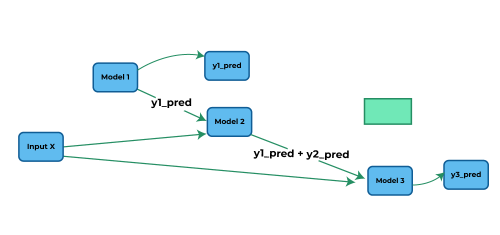
Chained regressionn

In this approach,

• Model 1 generates predictions (y1_pred) for Y1 using input X.
• Model 2 utilizes both y1_pred and X as input to make predictions for Y2 (y2_pred).
• Similarly, Model 3 takes y1_pred, y2_pred, and X as input to predict values for Y3 (y3_pred).

Python

from sklearn.multioutput import RegressorChain

# Defining the chained multioutput model
svm_chain = RegressorChain(SVR(kernel="rbf", C=100, gamma=0.1, epsilon=0.1))

svm_chain.fit(X_train,y_train)
showResults(y_test,svm_chain.predict(X_test))

Output:

R2 score:  0.9770183076559664
Mean squared error:  2.160857985360773
Mean absolute error:  0.8648991134909931
Predictions: 
|    Y1 |    Y2 |   Y1_pred |   Y2_pred |
|------:|------:|----------:|----------:|
| 16.47 | 16.9  |   15.4987 |   17.0196 |
| 13.17 | 16.39 |   12.9448 |   16.1628 |
| 32.82 | 32.78 |   32.2836 |   33.2849 |
| 41.32 | 46.23 |   41.6524 |   43.2883 |
| 16.69 | 19.76 |   17.0211 |   19.9793 |

Conclusion

In conclusion, we can say that multi-output regression provides a versatile framework for predicting multiple target variables, which is essential in various real-world applications. It can be approached in three main ways: first, by employing models which inherently support multi-output regression, using the MultiOutputRegressor to extend single-output models, and finally by using regression chains that consider dependencies among output variables. The choice of approach depends on the specific dataset and the nature of the problem.