ML | Non-Linear SVM
Last Updated :
01 Aug, 2023
Support Vector Machine (SVM) is one of the powerful and versatile machine learning algorithms that can be used for various applications like classification, regression, and outlier detection. It is capable of handling both linear and nonlinear data by finding an optimal hyperplane or decision boundary that maximizes the margin between different classes. SVMs (Support Vector Machines) do exceptionally well at handling high-dimensional feature spaces and successfully navigating complex data distributions. They work by identifying support vectors, which are the closest data points to the decision boundary, and use them to make predictions. SVMs are widely used in many fields due to their effectiveness and flexibility.
Both classification and regression tasks use the linear SVM (Support Vector Machine). In classification, it finds a hyperplane that has the greatest margin of separation between classes. For regression, the goal is to fit a linear function that predicts continuous target variables. However, in the real world, all of the data cannot be separated linearly and is impossible to fit with a linear kernel function. When dealing with intricate, nonlinear data distributions, requires nonlinear SVM with kernel functions. SVM which is nonlinear can capture complex correlations and patterns.
Non-Linear SVM
Nonlinear SVM (Support Vector Machine) is necessary when the data cannot be effectively separated by a linear decision boundary in the original feature space. Nonlinear SVM addresses this limitation by utilizing kernel functions to map the data into a higher-dimensional space where linear separation becomes possible. The kernel function computes the similarity between data points, allowing SVM to capture complex patterns and nonlinear relationships between features. This enables nonlinear SVM to handle intricate data distributions, such as curved or circular decision boundaries. By leveraging the kernel trick, nonlinear SVM provides a powerful tool for solving classification problems where linear separation is insufficient, extending its applicability to a wide range of real-world scenarios.
Key Concepts in Support Vector Machine
The key concept in Support Vector Machines is as follows:
- Hyperplane: Hyperplane is the decision boundary that is used to separate the data points of different classes in a feature space.
- Support Vectors: Support vectors are the data points closest to the decision boundary, which makes a critical role in deciding the hyperplane and margin.
- Margin: The margin is the distance between the decision boundary and the support vectors. SVM aims to maximize this margin to achieve better separation and generalization.
- Kernel: Kernel is a mathematical function used in SVM to map the original input data points into high-dimensional feature spaces, allowing the hyperplane to be located even when the data points are not linearly separable in the original input space. Radial basis function (RBF), linear, polynomial, and sigmoid are a few of the frequently used kernel functions.
- Nonlinear Decision Boundaries: Nonlinear SVM allows for the creation of complex decision boundaries that can accurately separate data points of different classes. By transforming the data using kernel functions, SVM can capture nonlinear relationships between features.
- Regularization Parameter: The regularization parameter (often denoted as C) controls the trade-off between the misclassification of training examples and the margin width. It helps prevent overfitting and influences the model’s complexity.
Support Vector Machines
The objective function of the Support Vector Machine is to find the optimal hyperplane that maximizes the margin between the two classes or best fits the data points in case of regression. The dual Problem of the optimization for support vector machine can be formulated as follows:

Where,
 is the Lagrange multiplier associated with each training example
  .
.- C is the regularization parameter that controls the trade-off between margin maximization and misclassification.
 is the kernel function that computes the similarity between training examples xi and xj.
Once the dual problem is solved and the optimal Lagrange multipliers are determined, the SVM decision boundary can be expressed in terms of these optimal Lagrange multipliers and the support vectors. The support vectors are the training samples with i > 0, and the decision boundary is given by:

Popular kernel functions in SVM
The SVM kernel is a function that transforms low-dimensional input space into higher-dimensional space, or in other words, it turns nonseparable problems into separable problems. It is most helpful in cases with non-linear separation. Simply explained, the kernel transforms data in a very complicated way before determining how to divide the data based on the labels or outputs specified.

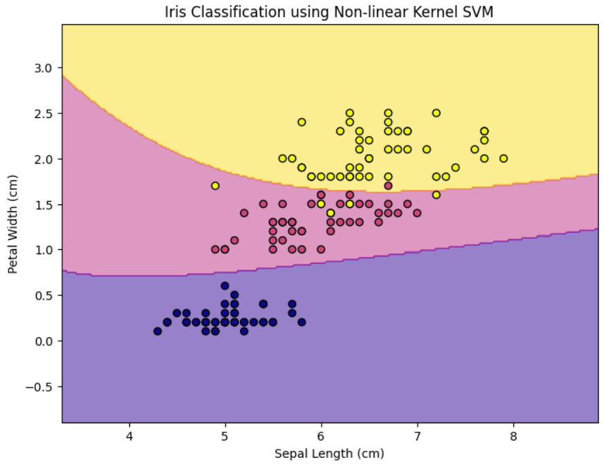
Example : Non-Linear SVM Classification
Let’s consider the example of the IRIS dataset plotted with only 2 of the 4 features (Sepal length and Petal Width). Following is the scatter plot of the same: It’s quite obvious that these classes are not linearly separable. Following is the contour plot of the non-linear SVM which has successfully classified the IRIS dataset using the Polynomial kernel with degree=5. The above figure shows the classification of the three classes of the IRIS dataset.
Below is the Python implementation for the same.
Python3
import numpy as np
import matplotlib.pyplot as plt
from sklearn.datasets import load_iris
from sklearn.svm import SVC
from sklearn.model_selection import train_test_split
iris = load_iris(as_frame=True)
df = iris.frame
X = df[['sepal length (cm)','petal width (cm)']].values
y = df.target
X_train, X_test, y_train, y_test = train_test_split(X, y, test_size=0.2, random_state=42)
svm = SVC(kernel='poly',degree=5, random_state=42)
svm.fit(X_train, y_train)
x_min, x_max = X[:, 0].min() - 1, X[:, 0].max() + 1
y_min, y_max = X[:, 1].min() - 1, X[:, 1].max() + 1
xx, yy = np.meshgrid(np.arange(x_min, x_max, 0.02),
np.arange(y_min, y_max, 0.02))
Z = svm.predict(np.c_[xx.ravel(), yy.ravel()])
Z = Z.reshape(xx.shape)
plt.figure(figsize=(8, 6))
plt.contourf(xx, yy, Z, alpha=0.5, cmap='plasma')
plt.scatter(X[:, 0], X[:, 1], c=y, edgecolors='k', cmap='plasma')
plt.xlabel('Sepal Length (cm)')
plt.ylabel('Petal Width (cm)')
plt.title('Iris Classification using Non-linear Kernel SVM')
plt.show()
|
Output:
Non-linear Kernel SVM Classification
Share your thoughts in the comments
Please Login to comment...