How to Lock Formulas in Excel

Fed up with unintentionally messing up your Excel formulas and causing chaos in your meticulously designed spreadsheets? Don’t worry! Mastering the skill of locking formulas is your solution. In this brief tutorial, we’ll delve into the techniques to protect your calculations from unintended alterations, ensuring that your Excel wizardry remains undisturbed. Let’s jump into the straightforward practice of locking formulas and ensuring the security of your data sorcery.

In this article, we will discuss how to lock and protect the formulas within the Excel sheet along with an example.

Understanding Cell References

Before we explore the $ shortcut, it’s crucial to grasp the concept of cell references. In Excel formulas, cell references indicate which cells to include in calculations. There are three main types of cell references:

Relative References

These are the default references in Excel. When you copy and paste a formula to a new cell, the references adjust relative to the formula’s new position.

Absolute References

Unlike relative references, these references stay constant when you copy and paste a formula. You create an absolute reference by placing a $ symbol before the column letter and row number, like this: $A$1.

Mixed References

These references enable you to lock either the column or row, but not both. Create a mixed reference by adding a $ symbol before either the column letter or row number, such as $A1 or A$1.

How to Lock Formula in Excel with Dollar Sign

Step 1: Open the Spreadsheet

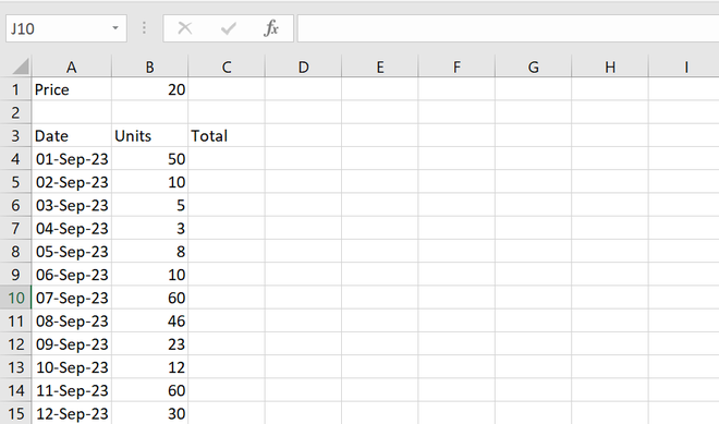
Open the sheet you want to lock formulas in.

Step 2: Lock the Formula Reference

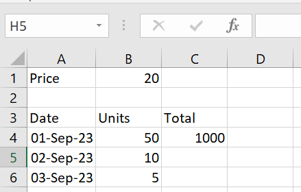
In this sheet we want to multiply the price with the units to calculate total units for every day.

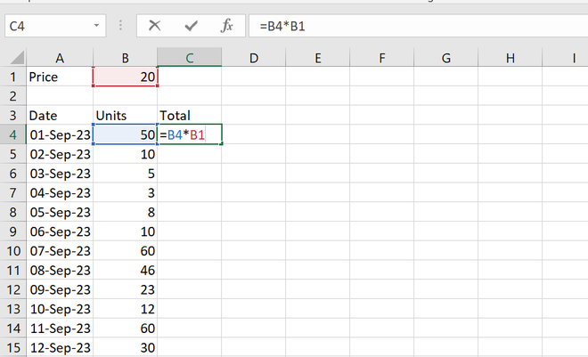
Enter the formula for one row as shown below.

Step 3: Locking the Reference to Cell B1

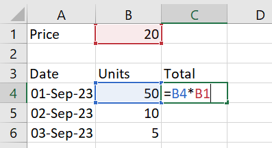
Now, we want to lock the reference to the cell “B1” because we want it to stay same for all the rows. When the formula is dragged the value of “B1” cell should remain the same.

Place the cursor at the end of B1 which is entered in the formula shown in the cell “C4” in the below image.

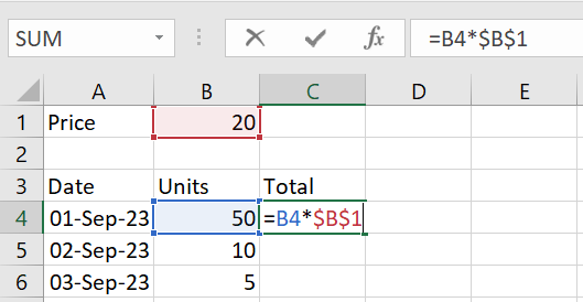
Press “F4”. You can confirm that the reference to the cell “B1” is locked when you see dollar sign($) placed in front of “B1” in the formula. As shown in the image below, like “$B$1”.

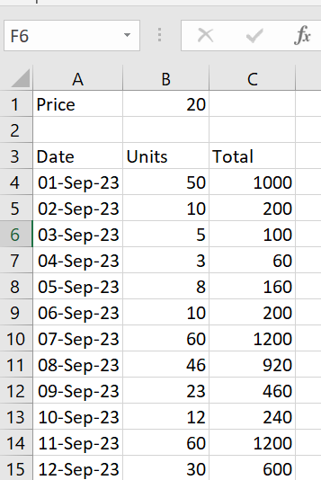
Step 4: Preview Result

Press “Enter”, you will see that the value is been calculated.

Step 5: Drag the formula to apply it to all the rows

How to Lock Formulas in Excel Without Protecting the Workbook

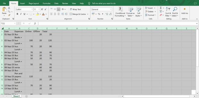
Step 1: Open the spreadsheet

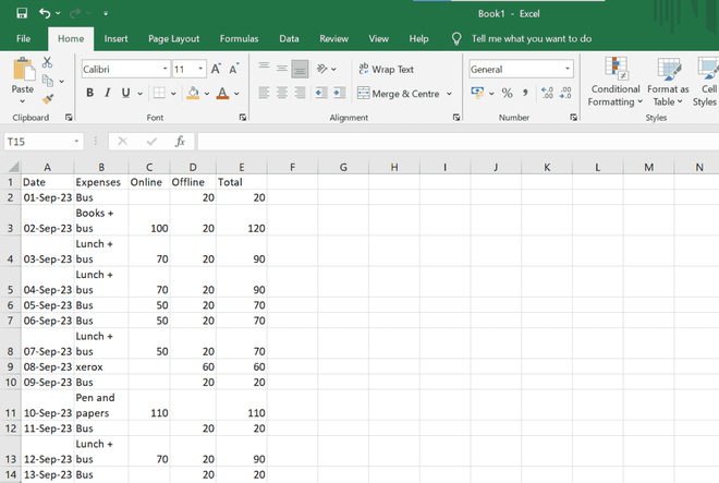
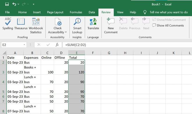
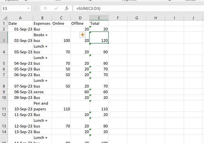
Suppose we have an Excel as follows which contains some calculations done with the help of formulas.

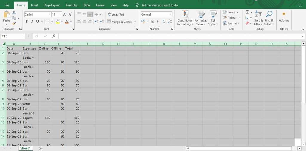
Step 2: Unlock all Cells

1. Select the whole excel sheet by pressing Ctrl + A.

Step 3: Right- Click and Select Format Cells

Right click while the cells are selected. Click on “Format Cells” option or Press Ctrl + 1.

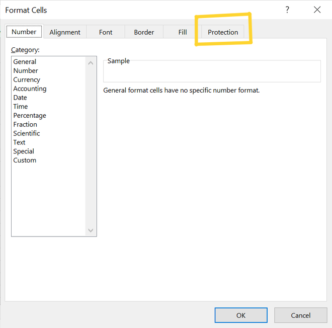
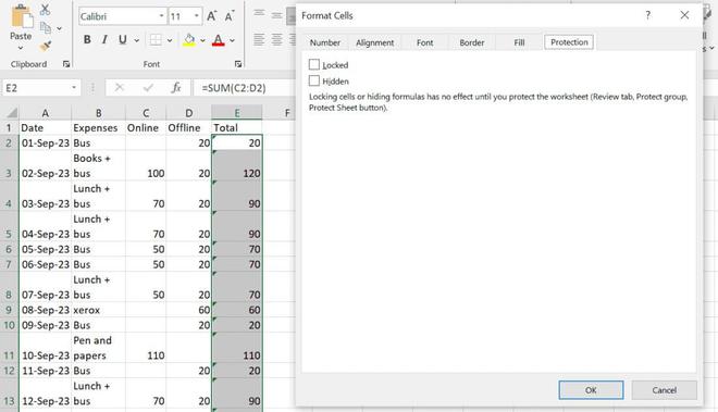
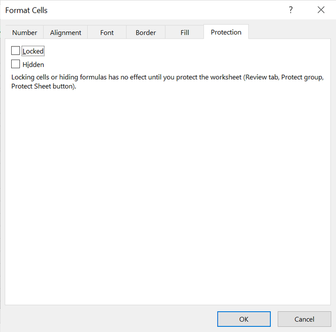
Step 4: Go to the Protection Tab

The below box will now open. Choose the “Protection” tab.

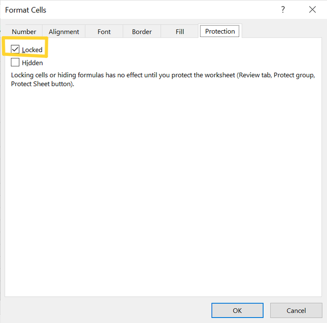
Step 5: Unmark the Locked Checkbox and Click Ok

Observe the “Locked” option is marked. Unmark this checkbox

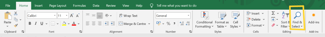
Step 6: Select the cells with formulas

1. Next go to the “Home” section. Select “Find & Select” option.

2. Completing the above step will open a dialog box as shown below. Click on “Go to Special”.

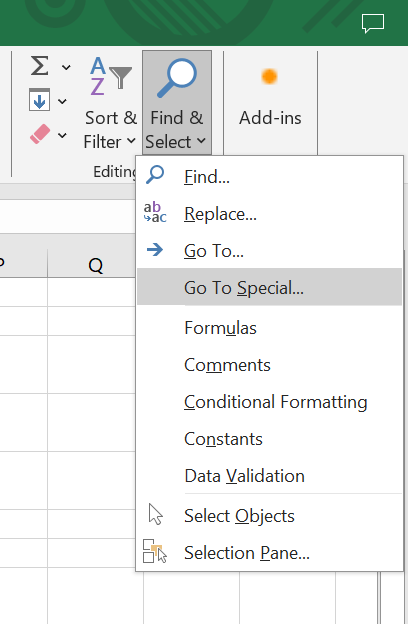
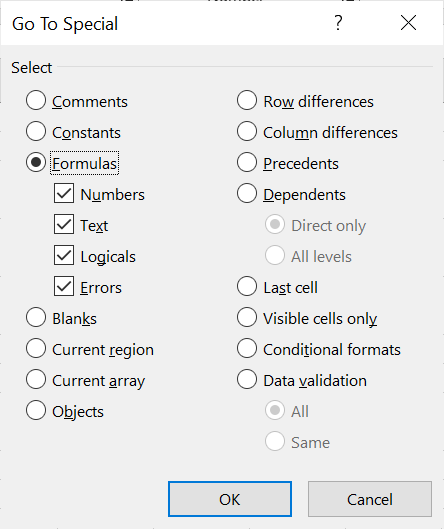
3. This will open a separate dialog box as shown below.

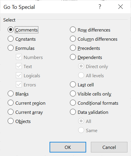
4. Choose the “Formulas” option. Click “Ok”.

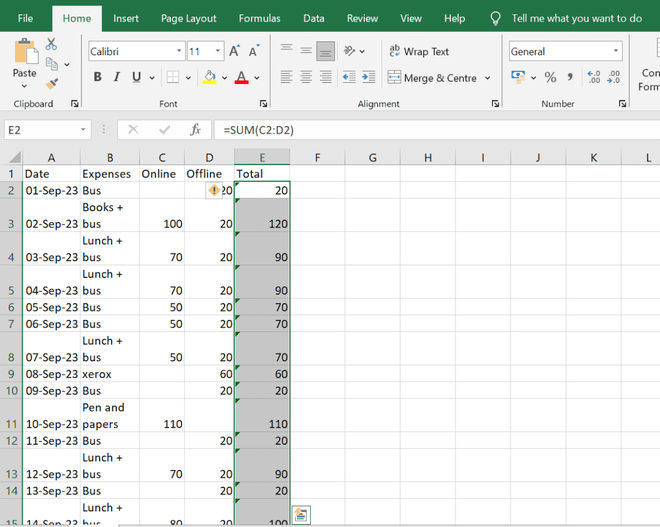
5. After the above step. All the cells containing formulas will be selected as shown below.

Step 7: Lock the cells

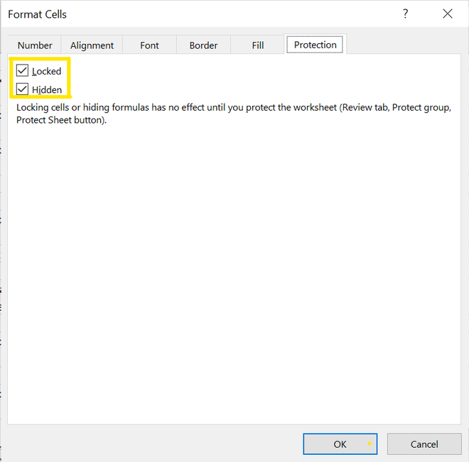
1. Now press Ctrl + 1. In the “Protection” tab check the “Locked” and “Hidden” option.

2. The options will look as below. Click “Ok”. All the cells containing formulas are now locked and hidden.

Step 8: Protect the cells

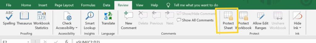
1. While the all the locked formula cells are still selected. Go to “Review” section.

2. Choose the “Protect Sheet” option.

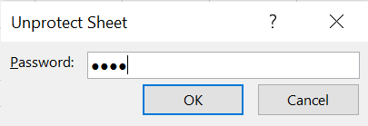
3. Now in the “Protect Sheet” dialog box, enter a password to secure the sheet. After you have entered the password click “Ok”.

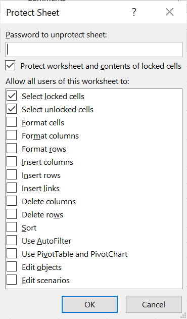
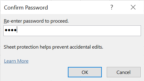
4. Confirm the password by re-entering it. Click on “Ok”.

The formulas are now safe and protected. You are free to make changes to any of the cells as you like. However, if you attempt to edit the cells that have the formulas, a message box will appear a shown below.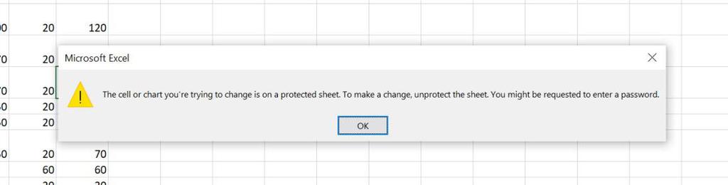

How to Lock Formulas in Excel shortcut

Step 1: Select the Cell

Select the cell with the formula you want to lock.

Step 2: Lock Formula’s cell reference

Press “F4” on the keyboard to lock the cell reference of the formula.

Step 3: Repeat the process

Repeat the process for all the other cells with formulas you want to lock.

How to Remove Protection and Unhide Formulas in Excel

Step 1: Open the spreadsheet

Step 2: Unprotect the cells

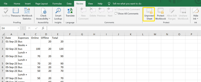
1. Go to the “Review” section. Click on “Unprotect Sheet” option.

2. After completing the above step the below dialog box will open.

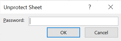
3. Enter the password you provided during protecting the cells.

Now the cells are unprotected.

Step 3: Unhide the formulas

1. Press Ctrl + A to select all the cells of the sheet.

2. Right click and select the “Format cells” option.

3. On the popped-up dialog box, go to “Protection” tab. Uncheck the “Locked” and “Hidden” option to unhide the formulas. Click on “Ok”.

Now the formulas are unhidden and unlocked.

Conclusion

You can use the above methods to lock and hide the formulas and secure the sheet from the unintentional changes. Steps are as well provided to unprotect the sheet and unhide the formulas.

FAQs

How do I lock formulas in Excel but allow data entry?

To lock formulas in Excel while still permitting data entry, select the cells containing the formulas that you want to protect. Right-click on the selected cells and choose “Format Cells.” In the “Format Cells” dialog box, go to the “Protection” tab. Uncheck the “Locked” option, which will prevent these cells from being locked by default. Click “OK” to confirm the changes. Next, go to the “Review” tab in Excel and click on “Protect Sheet.” In the “Protect Sheet” dialog box, you can set a password if you want to restrict access further. Make sure to check the “Select locked cells” and “Select unlocked cells” options to allow data entry in the unlocked cells. Click “OK” and enter the password if you’ve set one. Now, your formulas are protected, and users can only enter data in the unlocked cells while being unable to edit or view the formulas in the locked cells.

How do I lock certain formula cells in Excel?

Yes, you can lock formulas in specific cells only. To do this, you need to select the cells that contain the formulas you want to lock, and then press Ctrl + 1 to open the Format Cells dialog box. From there, go to the Protection tab and check the box next to “Locked”. Then, go to the Review tab, click the “Protect Sheet” you can set a password if you want to restrict access further, and check the box next to “Protect worksheet and contents of locked cells”. Click “OK” and enter the password if you’ve set one.

How do I lock a formula in Excel using F4?

To lock a formula in Excel using the F4 key, select the cell containing the formula you want to lock. Click on the formula within the formula bar or directly within the cell to place the cursor in the formula. Press the “F4” key on your keyboard. This will toggle between different reference styles, such as relative references (A1), absolute references with a dollar sign before the column and row ($A$1), and mixed references with either the column or the row locked ($A1 or A$1). Press “Enter” to lock the formula reference.

Can I lock the formulas in Excel without protecting the sheet?

Yes, you can lock the formulas in Excel without protecting the entire sheet by, selecting the cells containing the formulas that you want to lock. Right-click on the selected cells and choose “Format Cells.” In the “Format Cells” dialog box, go to the “Protection” tab. Uncheck the “Locked” option, which will prevent these cells from being locked by default. Click “OK” to confirm the changes. Go to the “Review” tab in Excel and click on “Allow Users to Edit Ranges”. In the “Allow Users to Edit Ranges” or “Range Permissions” dialog box, click “New” to define a new range. Select the cells that contain your formulas. These cells should be unlocked, as you unchecked the “Locked” option earlier. Click “Permissions” and set the password and any other settings you desire. Click “OK” to confirm the range permissions.