Highlight Rows Based on a Cell Value in Excel

Conditional Formatting generally checks the value in one cell and applies formatting over the other cells. A great application of conditional formatting is highlighting the entire row or multiple rows based on a cell value and condition provided in the formula.

 It is very helpful because for a data set with tons of value in it becomes cumbersome to analyze just by reading the data. So, if we highlight a few rows based on some conditions, it becomes easier for the user to infer from the data set. For example, in a college, some students have been blacklisted due to some illegal activities. So, in the Excel record the administrator can highlight the rows where these students records are present.

In this article we are going to see how to highlight row(s) based on cell value(s) using a suitable real time example shown below :

Example : Consider a company’s employees data is present. The following table consists of data about the project(s) which has been assigned to employees, their ages and ID. An employee can work on multiple projects. The blank cell in project denotes that no project has been assigned to that employee.

Highlighting the Rows

1. On the basis of text match : 

Aim : Highlight all the rows where Employee name is “Srishti”.

Steps :

1. Select the entire dataset from A3 to D14 in our case.

2. In the Home Tab select Conditional Formatting. A drop-down menu opens.

3. Select New Rule from the drop-down. The dialog box opens.

4. In the New Formatting Rule dialog box select “Use a Formula to determine which cells to format” in the Select a Rule Type option.

5. In the formula box, write the formula :

=$B2="Srishti"

$ is used to lock the column B, so that only the cell B is looked starting from Row 2

The formula will initially check if the name “Srishti” is present or not in the cell B2. Now, since cell B is locked and next time checking will be done from cell B3 and so on until the condition gets matched.

6. In the Preview field, select Format and then go to Fill and then select an appropriate color for highlighting and click OK

7. Now click OK and the rows will be highlighted.

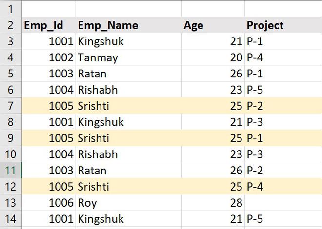
Highlighted Rows

2. Non-text matching based on number :

Aim : Highlight all the rows having age less than 25.

Approach :

Repeat the above steps as discussed and in the formula write :

=$C3<25

Highlighted Rows

3. On the basis of OR/AND condition :

OR, AND are used when we have multiple conditions. These are logical operators which work on True value.

AND : If all conditions are TRUE, AND returns TRUE.

OR : At least one of the conditions needs to be TRUE to return TRUE value.

Aim :  Highlight all the rows of employees who are either working on Project 1 or Project 4.

The project details are in column D. So, the formula will be :

=OR($D3="P-1",$D3="P-4")

Aim : Suppose employee Rishabh has completed the project P-3. The administrator is asked to highlight the row and keep a record of projects which are finished.

The name is in column B and the project details is in column D. The formula will be :

=AND($B3="Rishabh",$D3="P-3")

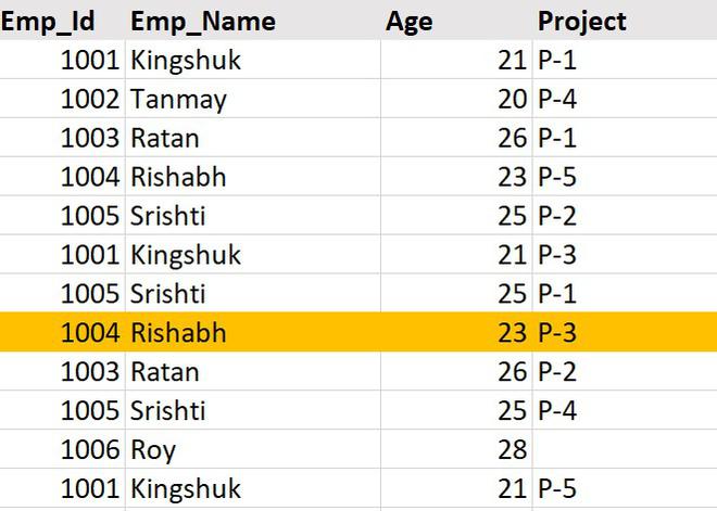
Highlighted Row

4. On the basis of any blank row :

Aim : Check if there is/are any blank row(s). If exist(s), then highlight it.

The project details is in column D. We will use the COUNTIF( ) function to check for the number of blank records. The formula will be :

=COUNTIF($A3:$D3,"")>0

"" : Denotes blank

The above formula checks all the columns one by one and sees if there is at least one blank row. If the formula value is greater than zero then highlighting will be done else COUNTIF will return FALSE value and no highlighting will be done.

5. On the basis of multiple conditions and each condition having different color :

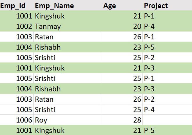
Aim : Suppose the company wants to distinguish the employees based on their ages. The employees whose age is more than 25 are senior employees and whose age is more than 20 but less than or equal to 25 are junior developers or trainees. So, the administrator is asked to highlight these two categories with different colors.

Implementation :

In the Formula Field write the formula :

=$C3>25

This will highlight all the rows where age is more than 25.

Again in the Formula Field write the formula :

=$C3>20

This will highlight all the rows greater than 20. It will in fact change the color of the rows where age is greater than 25. Since, if a number is greater than 20 then definitely it is greater than 25. So, all the cells having age more than 20 will be highlighted to the same color. 

This creates a problem as our goal is to make two separate groups. In order to resolve this we need to change the priority of highlighting the rows. The steps are :

• Undo the previous steps using CTRL+Z.
• Select the entire dataset.
• Go to Conditional Formatting followed by Manage Rules.

• In the Manage Rule dialog box :

The order of the condition needs to be changed. The condition at the top will have more priority than the lower one. So, we need to move the second condition to the top of the first one using the up icon after selecting the condition.

• Now click on Apply and then OK. 

It can be observed that the rows are now divided into two categories : The yellow color is for the senior level employees and the green color is for junior employees and trainees in the company on the basis of their ages.