Factorial Design in R

Factorial designs are powerful tools in experimental design, allowing researchers to efficiently explore the effects of multiple factors and their interactions on a response variable.

In R Programming Language various packages offer capabilities to create, manipulate, and analyze factorial designs. Here, we’ll explore the fundamentals of factorial designs and demonstrate how to implement them using R.

What is Factorial Design?

Factorial design involves studying the impact of multiple factors simultaneously. Each factor can have multiple levels, and the combinations of these levels form the experimental conditions. This design helps in understanding the main effects of individual factors and their interactions on the response variable.

Factorial designs in R typically rely on several packages that provide specific functionalities:

• stats: Offers foundational tools for data manipulation, statistical modeling (like lm for linear regression), and basic design creation (e.g., expand. grid).
• DoE.base: Provides a comprehensive framework for designing experiments, including full and fractional factorial designs, response surface methodologies, and more advanced experimental designs.
• FrF2: Specifically used for creating regular and non-regular factorial designs, particularly fractional factorial designs of 2^k and 3^k types.
• DAAG: Offers functions and datasets for design and analysis, focusing on experimental designs for teaching and research.

Important Parts of Factorial Design

1. Factors and Levels- Factors are the things which change, like temperature or time and Levels are the different settings or values of these factors.
2. Treatment Combinations- Shows all the different mixes of factors which test together, creating specific conditions for experiments.
3. Main Effects and Interactions- Checks how each factor alone affects the result (main effect) and how they change when paired up (interaction).
4. Response Variable- This is what we’re watching for changes – like plant growth or product quality when we adjust factors.
5. Factorial Notation– Uses numbers like 2³ to quickly show how many factors and levels we’re dealing with.
6. Efficiency in Experimentation– Getting lots of info from fewer tests, saving time and resources while keeping errors low.
7. Analysis and Interpretation– Using math tools to make sense of results, figuring out what the numbers mean for our experiment.

Types of Factorial Design

2^k Factorial Design

Examines the effects of k factors at two levels each.

R

# Install and load the FrF2 package if not installed
install.packages("FrF2")
library(FrF2)

# Creating a 2^2 factorial design with a resolution of 3
design_2k <- FrF2(nfactors = 2, resolution = 3)
print(design_2k)

Output:

   A  B
1  1  1
2 -1 -1
3 -1  1
4  1 -1
class=design, type= full factorial 

This will generate a 2^2 factorial design with two factors at two levels each.

Factorial Design with Fractional Factorial

Investigates a subset of factor combinations to reduce the number of runs.

R

library(DoE.base) # Load the package
# Creating a fractional factorial design with 4 factors and 8 runs
design_frac <- oa.design(nfactors = 4, nlevels = 2, nruns = 8)
print(design_frac)

Output:

  A B C D
1 2 2 2 2
2 1 2 2 1
3 1 1 2 2
4 2 1 2 1
5 1 1 1 1
6 1 2 1 2
7 2 1 1 2
8 2 2 1 1
class=design, type= oa 

Plackett-Burman Design

Used for screening a large number of factors to identify the most influential ones.

R

# Load the necessary package
library(FrF2)

# Creating a Plackett-Burman design with 7 factors
design_PB <- pb(nruns = 8, nfactors = 7)
print(design_PB)

Output:

   A  B  C  D  E  F  G
1 -1  1 -1 -1  1  1  1
2 -1 -1  1  1  1 -1  1
3  1 -1  1 -1 -1  1  1
4 -1  1  1  1 -1  1 -1
5  1  1 -1  1 -1 -1  1
6  1  1  1 -1  1 -1 -1
7  1 -1 -1  1  1  1 -1
8 -1 -1 -1 -1 -1 -1 -1
class=design, type= pb 

Difference Between the Types of Factorial Design

Aspect	2^k Factorial Design	Fractional Factorial Design	Plackett-Burman Design
Factors	Examines k factors	Examines a subset of factors	Screens main effects of factors
Levels per Factor	Typically two levels per factor	Typically two levels per factor	Typically two levels per factor
Number of Runs	2k runs	Fewer runs than run 2k	Depends on the number of factors
Resolution	Depends on k (low to high)	Usually lower resolution (subsets)	Not adjustable, full resolution
Purpose	Study main effects and interactions	Identify influential factors	Screen factors for main effects
Efficiency in Factor Screening	Less efficient for many factors	Efficient for many factors	Efficient for a few factors
Design Flexibility	Provides full factorial information	Provides reduced information	Provides reduced information

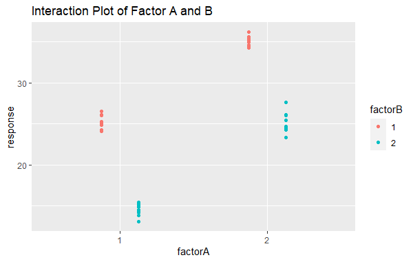
Visualization

R

# Generating a sample factorial design data
factorA <- factor(rep(1:2, each = 20))
factorB <- factor(rep(1:2, times = 20))
response <- rnorm(40, mean = c(20, 30)[factorA] + c(5, -5)[factorB])

# Creating a data frame
data <- data.frame(factorA, factorB, response)

# Interaction plot
library(ggplot2)
ggplot(data, aes(x = factorA, y = response, color = factorB)) +
  geom_point(position = position_dodge(width = 0.5)) +
  labs(title = "Interaction Plot of Factor A and B")

Output:

Factorial Design in R

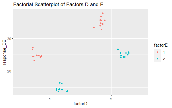
Factorial Scatterplot

R

# Generating a sample factorial design data
factorD <- factor(rep(1:2, times = 20))
factorE <- factor(rep(1:2, each = 20))
response_DE <- rnorm(40, mean = c(20, 30)[factorD] + c(5, -5)[factorE])

# Creating a data frame
data_DE <- data.frame(factorD, factorE, response_DE)

# Factorial scatterplot
library(ggplot2)
ggplot(data_DE, aes(x = factorD, y = response_DE, color = factorE)) +
  geom_point(position = position_jitterdodge()) +
  labs(title = "Factorial Scatterplot of Factors D and E")

Output:

Factorial Design in R

Visualizes the relationships between multiple factors and the response.

Benefits of Factorial Design

• Understanding Many Things Together -Helps study lots of factors at the same time, showing how they work together.
• Saving Time and Money -Gives lots of information with fewer experiments, saving time and resources.
• Finding Connections -Reveals hidden ways factors influence each other, finding connections we might miss otherwise.
• Better Decision-Making -Helps make smarter decisions by showing which factors really matter in an experiment.
• Efficient Experimenting -Does a lot with only a few tests, making experiments more efficient.

Implementing Factorial Designs in R

1)Using the “stats” Package

The stats package provides a basic framework to create factorial designs using functions like expand.grid and perform analysis with statistical models such as linear regression (lm) or ANOVA (anova).

Step 1: Install and Load Required Packages

R

library(stats)

Step 2: Generate a 2 x 2 Fractional Factorial Design

R

# Create a simple 2x2 factorial design
design <- expand.grid(factor1 = c("A", "B"),
                      factor2 = c("X", "Y"))

Step 3: Add Response Variables

R

design$response <- rnorm(nrow(design))  # Generating random response values

# Display the design
print(design)

Output:

  factor1 factor2   response
1       A       X  1.6640891
2       B       X -0.6159014
3       A       Y -0.3310070
4       B       Y  0.6026683

Step 4: Analyze the Design using Linear Regression

R

# Fit a linear model and perform ANOVA
model <- lm(response ~ factor1 * factor2, data = design)
anova_result <- anova(model)
print(anova_result)

Output:

Analysis of Variance Table

Response: response
                Df  Sum Sq Mean Sq F value Pr(>F)
factor1          1 0.45314 0.45314     NaN    NaN
factor2          1 0.15075 0.15075     NaN    NaN
factor1:factor2  1 2.58191 2.58191     NaN    NaN
Residuals        0 0.00000     NaN     

Using the “FrF2” package

Showcase the FrF2 package for creating regular and non-regular factorial designs, especially fractional factorial designs.

Here’s a step by step approach of FrF2 package

Step 1: Install and Load Required Packages

If you haven’t already installed the FrF2 package, you can install it and load it into R.

R

# Install if not already installed
install.packages("FrF2")

# Load necessary packages
library(FrF2)

Step 2: Generate a 2³ Fractional Factorial Design

R

# Generating a 2^3 fractional factorial design
design_2k <- FrF2(nfactors = 3, resolution = 3)
print(design_2k)

Output:

   A  B  C
1 -1 -1  1
2  1  1  1
3  1 -1 -1
4 -1  1 -1
class=design, type= FrF2 

This code generates a 2³ fractional factorial design with three factors at a resolution of 3 and prints the design matrix.

Step 3: Add Response Variables

R

# Add a response variable
design_2k$response <- rnorm(nrow(design_2k))

For demonstration purposes, add a response variable to the generated design. Here, random response values are generated.

Step 4: Analyze the Design using Linear Regression

Fit a linear regression model to analyze the effect of factors on the response variable.

R

# Fit a linear regression model
model <- lm(response ~ ., data = design_2k)
summary(model)

Output:

Call:
lm.default(formula = response ~ ., data = design_2k)

Residuals:
ALL 4 residuals are 0: no residual degrees of freedom!

Coefficients:
            Estimate Std. Error t value Pr(>|t|)
(Intercept)  0.13528        NaN     NaN      NaN
A1          -0.05577        NaN     NaN      NaN
B1           0.11630        NaN     NaN      NaN
C1           0.92214        NaN     NaN      NaN

Residual standard error: NaN on 0 degrees of freedom
Multiple R-squared:      1,    Adjusted R-squared:    NaN 
F-statistic:   NaN on 3 and 0 DF,  p-value: NA

This code uses the lm function to fit a linear regression model, where the response variable (response) is predicted by all the factors in the design. The summary function provides information about the coefficients, significance, and goodness of fit of the model

Practical Application Example

Let’s say you’re a baker testing new cake recipes. You want to understand how different factors—like flour type (A) and baking temperature (B)—affect the cake’s height (the response variable).

Factorial Design Approach

Factor A (Flour Type):

• Levels: Regular flour vs. gluten-free flour.

Factor B (Baking Temperature):

• Levels: Low temperature (350°F) vs. high temperature (400°F).

How Factorial Design Helps

1. Efficient Testing: With a 2×2 factorial design, you can bake cakes using all combinations: Regular flour at low temperature, regular flour at high temperature, gluten-free flour at low temperature, and gluten-free flour at high temperature.
2. Understanding Interactions: This design allows you to see how flour type and temperature interact. For instance, does gluten-free flour rise differently at high temperatures compared to regular flour?
3. Identifying Main Effects: Let’s observe how each factor affects the cake’s height individually. Is there a significant difference in height between regular and gluten-free flour? Does temperature impact height regardless of flour type?
4. Optimization: By analyzing the results, you might find that one flour type rises better at a specific temperature. This knowledge can help optimize the recipe for the tallest cakes.

Factorial designs help bakers systematically test various combinations of factors, understanding their individual impacts and interactions. This approach efficiently guides recipe development by identifying the best combinations for the tallest, most appealing cakes.

Conclusion

Factorial designs in R offer a powerful way to explore how different factors influence outcomes in experiments. With packages like “stats”, “FrF2”, and others, researchers can efficiently create, manipulate, and analyze these designs. By examining multiple factors simultaneously, we uncover not just their individual effects but also how they interact, providing deeper insights into complex relationships. These designs streamline experimentation, making it easier to optimize outcomes, understand interactions, and draw meaningful conclusions from data.