A decision tree in machine learning is a versatile, interpretable algorithm used for predictive modelling. It structures decisions based on input data, making it suitable for both classification and regression tasks. This article delves into the components, terminologies, construction, and advantages of decision trees, exploring their applications and learning algorithms.
Decision Tree in Machine Learning
A decision tree is a type of supervised learning algorithm that is commonly used in machine learning to model and predict outcomes based on input data. It is a tree-like structure where each internal node tests on attribute, each branch corresponds to attribute value and each leaf node represents the final decision or prediction. The decision tree algorithm falls under the category of supervised learning. They can be used to solve both regression and classification problems.
Decision Tree Terminologies
There are specialized terms associated with decision trees that denote various components and facets of the tree structure and decision-making procedure. :
- Root Node: A decision tree’s root node, which represents the original choice or feature from which the tree branches, is the highest node.
- Internal Nodes (Decision Nodes): Nodes in the tree whose choices are determined by the values of particular attributes. There are branches on these nodes that go to other nodes.
- Leaf Nodes (Terminal Nodes): The branches’ termini, when choices or forecasts are decided upon. There are no more branches on leaf nodes.
- Branches (Edges): Links between nodes that show how decisions are made in response to particular circumstances.
- Splitting: The process of dividing a node into two or more sub-nodes based on a decision criterion. It involves selecting a feature and a threshold to create subsets of data.
- Parent Node: A node that is split into child nodes. The original node from which a split originates.
- Child Node: Nodes created as a result of a split from a parent node.
- Decision Criterion: The rule or condition used to determine how the data should be split at a decision node. It involves comparing feature values against a threshold.
- Pruning: The process of removing branches or nodes from a decision tree to improve its generalisation and prevent overfitting.
Understanding these terminologies is crucial for interpreting and working with decision trees in machine learning applications.
How Decision Tree is formed?
The process of forming a decision tree involves recursively partitioning the data based on the values of different attributes. The algorithm selects the best attribute to split the data at each internal node, based on certain criteria such as information gain or Gini impurity. This splitting process continues until a stopping criterion is met, such as reaching a maximum depth or having a minimum number of instances in a leaf node.
Why Decision Tree?
Decision trees are widely used in machine learning for a number of reasons:
- Decision trees are so versatile in simulating intricate decision-making processes, because of their interpretability and versatility.
- Their portrayal of complex choice scenarios that take into account a variety of causes and outcomes is made possible by their hierarchical structure.
- They provide comprehensible insights into the decision logic, decision trees are especially helpful for tasks involving categorisation and regression.
- They are proficient with both numerical and categorical data, and they can easily adapt to a variety of datasets thanks to their autonomous feature selection capability.
- Decision trees also provide simple visualization, which helps to comprehend and elucidate the underlying decision processes in a model.
Decision Tree Approach
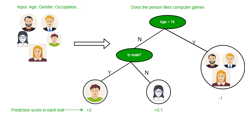
Decision tree uses the tree representation to solve the problem in which each leaf node corresponds to a class label and attributes are represented on the internal node of the tree. We can represent any boolean function on discrete attributes using the decision tree.
Below are some assumptions that we made while using the decision tree:
At the beginning, we consider the whole training set as the root.
- Feature values are preferred to be categorical. If the values are continuous then they are discretized prior to building the model.
- On the basis of attribute values, records are distributed recursively.
- We use statistical methods for ordering attributes as root or the internal node.
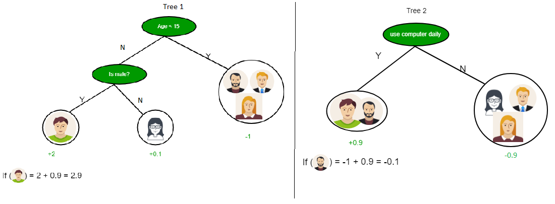
As you can see from the above image the Decision Tree works on the Sum of Product form which is also known as Disjunctive Normal Form. In the above image, we are predicting the use of computer in the daily life of people. In the Decision Tree, the major challenge is the identification of the attribute for the root node at each level. This process is known as attribute selection. We have two popular attribute selection measures:
- Information Gain
- Gini Index
1. Information Gain:
When we use a node in a decision tree to partition the training instances into smaller subsets the entropy changes. Information gain is a measure of this change in entropy.
- Suppose S is a set of instances,
- A is an attribute
- Sv is the subset of S
- v represents an individual value that the attribute A can take and Values (A) is the set of all possible values of A, then

Entropy: is the measure of uncertainty of a random variable, it characterizes the impurity of an arbitrary collection of examples. The higher the entropy more the information content.
Suppose S is a set of instances, A is an attribute, Sv is the subset of S with A = v, and Values (A) is the set of all possible values of A, then

Example:
For the set X = {a,a,a,b,b,b,b,b}
Total instances: 8
Instances of b: 5
Instances of a: 3
![\begin{aligned} \text{Entropy } H(X) & =\left [ \left ( \frac{3}{8} \right )\log_{2}\frac{3}{8} + \left ( \frac{5}{8} \right )\log_{2}\frac{5}{8} \right ] \\& = -[0.375 (-1.415) + 0.625 (-0.678)] \\& = -(-0.53-0.424) \\& = 0.954 \end{aligned}](https://quicklatex.com/cache3/34/ql_5fde2759a2fefb3453e413bb1ddb3834_l3.png "Rendered by QuickLaTeX.com")
Building Decision Tree using Information Gain The essentials:
- Start with all training instances associated with the root node
- Use info gain to choose which attribute to label each node with
- Note: No root-to-leaf path should contain the same discrete attribute twice
- Recursively construct each subtree on the subset of training instances that would be classified down that path in the tree.
- If all positive or all negative training instances remain, the label that node “yes” or “no” accordingly
- If no attributes remain, label with a majority vote of training instances left at that node
- If no instances remain, label with a majority vote of the parent’s training instances.
Example: Now, let us draw a Decision Tree for the following data using Information gain. Training set: 3 features and 2 classes
Here, we have 3 features and 2 output classes. To build a decision tree using Information gain. We will take each of the features and calculate the information for each feature. 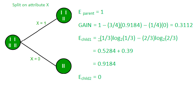
Split on feature X

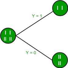
Split on feature Y
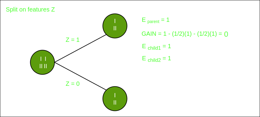
Split on feature Z
From the above images, we can see that the information gain is maximum when we make a split on feature Y. So, for the root node best-suited feature is feature Y. Now we can see that while splitting the dataset by feature Y, the child contains a pure subset of the target variable. So we don’t need to further split the dataset. The final tree for the above dataset would look like this:
2. Gini Index
- Gini Index is a metric to measure how often a randomly chosen element would be incorrectly identified.
- It means an attribute with a lower Gini index should be preferred.
- Sklearn supports “Gini” criteria for Gini Index and by default, it takes “gini” value.
- The Formula for the calculation of the Gini Index is given below.
The Formula for Gini Index is given by :

Gini Impurity
The Gini Index is a measure of the inequality or impurity of a distribution, commonly used in decision trees and other machine learning algorithms. It ranges from 0 to 0.5, where 0 indicates a pure set (all instances belong to the same class), and 0.5 indicates a maximally impure set (instances are evenly distributed across classes).
Some additional features and characteristics of the Gini Index are:
- It is calculated by summing the squared probabilities of each outcome in a distribution and subtracting the result from 1.
- A lower Gini Index indicates a more homogeneous or pure distribution, while a higher Gini Index indicates a more heterogeneous or impure distribution.
- In decision trees, the Gini Index is used to evaluate the quality of a split by measuring the difference between the impurity of the parent node and the weighted impurity of the child nodes.
- Compared to other impurity measures like entropy, the Gini Index is faster to compute and more sensitive to changes in class probabilities.
- One disadvantage of the Gini Index is that it tends to favour splits that create equally sized child nodes, even if they are not optimal for classification accuracy.
- In practice, the choice between using the Gini Index or other impurity measures depends on the specific problem and dataset, and often requires experimentation and tuning.
Example of a Decision Tree Algorithm
Forecasting Activities Using Weather Information
- Root node: Whole dataset
- Attribute : “Outlook” (sunny, cloudy, rainy).
- Subsets: Overcast, Rainy, and Sunny.
- Recursive Splitting: Divide the sunny subset even more according to humidity, for example.
- Leaf Nodes: Activities include “swimming,” “hiking,” and “staying inside.”
Beginning with the entire dataset as the root node of the decision tree:
- Determine the best attribute to split the dataset based on information gain, which is calculated by the formula: Information gain = Entropy(parent) – [Weighted average] * Entropy(children), where entropy is a measure of impurity or disorder of a set of examples, and the weighted average is based on the number of examples in each child node.
- Create a new internal node that corresponds to the best attribute and connects it to the root node. For example, if the best attribute is “outlook” (which can have values “sunny”, “overcast”, or “rainy”), we create a new node labeled “outlook” and connect it to the root node.
- Partition the dataset into subsets based on the values of the best attribute. For example, we create three subsets: one for instances where the outlook is “sunny”, one for instances where the outlook is “overcast”, and one for instances where the outlook is “rainy”.
- Recursively repeat steps 1-4 for each subset until all instances in a given subset belong to the same class or no further splitting is possible. For example, if the subset of instances where the outlook is “overcast” contains only instances where the activity is “hiking”, we assign a leaf node labeled “hiking” to this subset. If the subset of instances where the outlook is “sunny” is further split based on the humidity attribute, we repeat steps 2-4 for this subset.
- Assign a leaf node to each subset that contains instances that belong to the same class. For example, if the subset of instances where the outlook is “rainy” contains only instances where the activity is “stay inside”, we assign a leaf node labeled “stay inside” to this subset.
- Make predictions based on the decision tree by traversing it from the root node to a leaf node that corresponds to the instance being classified. For example, if the outlook is “sunny” and the humidity is “high”, we traverse the decision tree by following the “sunny” branch and then the “high humidity” branch, and we end up at a leaf node labeled “swimming”, which is our predicted activity.
Advantages of Decision Tree
- Easy to understand and interpret, making them accessible to non-experts.
- Handle both numerical and categorical data without requiring extensive preprocessing.
- Provides insights into feature importance for decision-making.
- Handle missing values and outliers without significant impact.
- Applicable to both classification and regression tasks.
Disadvantages of Decision Tree
- Disadvantages include the potential for overfitting
- Sensitivity to small changes in data, limited generalization if training data is not representative
- Potential bias in the presence of imbalanced data.
Conclusion
Decision trees, a key tool in machine learning, model and predict outcomes based on input data through a tree-like structure. They offer interpretability, versatility, and simple visualization, making them valuable for both categorization and regression tasks. While decision trees have advantages like ease of understanding, they may face challenges such as overfitting. Understanding their terminologies and formation process is essential for effective application in diverse scenarios.
Frequently Asked Questions (FAQs)
1. What are the major issues in decision tree learning?
Major issues in decision tree learning include overfitting, sensitivity to small data changes, and limited generalization. Ensuring proper pruning, tuning, and handling imbalanced data can help mitigate these challenges for more robust decision tree models.
2. How does decision tree help in decision making?
Decision trees aid decision-making by representing complex choices in a hierarchical structure. Each node tests specific attributes, guiding decisions based on data values. Leaf nodes provide final outcomes, offering a clear and interpretable path for decision analysis in machine learning.
3. What is the maximum depth of a decision tree?
The maximum depth of a decision tree is a hyperparameter that determines the maximum number of levels or nodes from the root to any leaf. It controls the complexity of the tree and helps prevent overfitting.
4. What is the concept of decision tree?
A decision tree is a supervised learning algorithm that models decisions based on input features. It forms a tree-like structure where each internal node represents a decision based on an attribute, leading to leaf nodes representing outcomes.
5. What is entropy in decision tree?
In decision trees, entropy is a measure of impurity or disorder within a dataset. It quantifies the uncertainty associated with classifying instances, guiding the algorithm to make informative splits for effective decision-making.
6. What are the Hyperparameters of decision tree?
- Max Depth: Maximum depth of the tree.
- Min Samples Split: Minimum samples required to split an internal node.
- Min Samples Leaf: Minimum samples required in a leaf node.
- Criterion: The function used to measure the quality of a split
Share your thoughts in the comments
Please Login to comment...