Coping with Missing, Invalid and Duplicate Data in R

Data is the base of statistical analysis and machine learning. The free data we get for processing is often raw and has many issues like invalid terms, and missing or duplicate values that can cause major changes in our model processing and estimation.

We use the past data to train our model and predict values based on this past data. These issues like invalid data or missing values can cause lower accuracy in prediction models therefore, handling these problems is an important part of data processing. In this article, we will learn how to cope with missing, invalid, and duplicate data in R Programming Language.

What is missing data?

Missing data is the missing values in the dataset that can cause issues in various predictions. Many statistical and machine learning models cannot handle such values, so it is important to handle them. To deal with missing values we must identify them first.

Identifying Missing Data

Before dealing with missing data we must identify them in the dataset. We can use is.na() function to identify missing values.

R

# Check for missing values in a data frame
missing_values <- is.na(my_data)

Once the missing data is identified we need to handle it.

How to Deal with Missing Data?

There are several ways to deal with the missing values such as deleting the rows and columns or imputing the unavailable values from the dataset. These ways are discussed below with the help of examples.

Deleting missing rows and columns

We can delete the rows and columns that have missing values. We can do it using the na.omit() function or complete.cases() functions as well.

R

# Remove rows with missing values
clean_data <- my_data[complete.cases(my_data), ]

We can also understand this with the help of an example. In this example, we will create a fictional dataset of ID, Age, and Salary and deal with the missing values in it.

R

# Creating a sample data frame with missing values
my_data <- data.frame(
  ID = c(1, 2, 3, 4, 5),
  Age = c(25, NA, 30, 22, 35),
  Salary = c(50000, 60000, NA, 45000, 70000)
)

# Display the original data frame
print("Original Data Frame:")
print(my_data)

# Applying na.omit() to remove rows with missing values
clean_data <- na.omit(my_data)

# Display the data frame after omitting missing values
print("Data Frame after using na.omit():")
print(clean_data)

Output:

[1] "Original Data Frame:"
  ID Age Salary
1  1  25  50000
2  2  NA  60000
3  3  30     NA
4  4  22  45000
5  5  35  70000

[1] "Data Frame after using na.omit():"
  ID Age Salary
1  1  25  50000
4  4  22  45000
5  5  35  70000

The rows and columns that had NA values are deleted in the output so that the missing values can not alter our predictions,

Imputing the missing values

We can also replace the missing values with the substituted values. Imputation in statistics is a technique by which we use substituted values in place of missing values to deal with them. These substituted values can be calculated with the help of the mean, median, or mode values of the dataset. The syntax to impute values is given below:

R

# Impute missing values with mean
my_data_imputed <- na.aggregate(my_data, FUN = mean)

We can understand this with the help of the same example mentioned above.

R

# Creating a sample data frame with missing values
my_data <- data.frame(
  ID = c(1, 2, 3, 4, 5),
  Age = c(25, NA, 30, 22, 35),
  Salary = c(50000, 60000, NA, 45000, 70000)
)

# Display the original data frame
print("Original Data Frame:")
print(my_data)

# Imputing missing values with mean
imputed_data <- my_data

# Impute Age column with mean
imputed_data$Age <- ifelse(is.na(imputed_data$Age), mean(imputed_data$Age,
                                                        na.rm = TRUE), imputed_data$Age)

# Impute Salary column with mean
imputed_data$Salary <- ifelse(is.na(imputed_data$Salary),
                              mean(imputed_data$Salary, na.rm = TRUE),
                              imputed_data$Salary)

# Display the data frame after imputation
print("Data Frame after Imputation:")
print(imputed_data)

Output:

[1] "Original Data Frame:"
  ID Age Salary
1  1  25  50000
2  2  NA  60000
3  3  30     NA
4  4  22  45000
5  5  35  70000

[1] "Data Frame after Imputation:"
  ID Age Salary
1  1  25  50000
2  2  28  60000
3  3  30  56250
4  4  22  45000
5  5  35  70000

Here, we replace the values with the mean values of the dataset.

Interpolation of missing data

We can also replace the missing values with the help of an estimation of the other points that are available to us. This is known as interpolation. For this, we need to install the zoo package in R.

Syntax:

R

#install library
install.packages("zoo")
#load package
library(zoo)

# Interpolate missing values
my_data_interp <- zoo::na.approx(my_data)

Applying this to the above-mentioned example we will get:

R

# Interpolate missing values using na.approx from zoo
interpolated_data <- my_data

# Interpolate Age column
interpolated_data$Age <- zoo::na.approx(interpolated_data$Age)

# Interpolate Salary column
interpolated_data$Salary <- zoo::na.approx(interpolated_data$Salary)

# Display the data frame after interpolation
print("Data Frame after Interpolation:")
print(interpolated_data)

Output:

[1] "Data Frame after Interpolation:"
  ID  Age Salary
1  1 25.0  50000
2  2 27.5  60000
3  3 30.0  52500
4  4 22.0  45000
5  5 35.0  70000

The missing values in our original dataset are now replaced with the estimated points based on the data set we have. We use the na.approx function to interpolate missing values in the Age and Salary columns.

What is Invalid Data?

Invalid data is data that does not fit with the given range or format of the given dataset. Some values in the column or row can have a different nature from the column, such data is known as invalid.

Identifying Invalid data

To deal with invalid data we must identify it first. To identify the invalid data we need to look for outliers, data types, or ranges. To check the data type for a new example of the “mtcars” data set that is inbuilt in R. We can use the following syntax to create an invalid dataset:

R

# Create a new example dataset with issues
my_data_invalid <- mtcars

# Introduce issues: modify data types, add outliers, and change some values
# introduce character data in a numeric column
my_data_invalid$mpg[1] <- "abc"
# introduce character data in a numeric column
my_data_invalid$hp[3] <- "xyz"
# introduce an outlier
my_data_invalid$mpg[5] <- 45
# introduce an outlier
my_data_invalid$mpg[10] <- 35

# Display the dataset with issues
print("Dataset with Issues:")
print(my_data_invalid)

Output:

[1] "Dataset with Issues:"
                     mpg cyl  disp  hp drat    wt  qsec vs am gear carb
Mazda RX4            abc   6 160.0 110 3.90 2.620 16.46  0  1    4    4
Mazda RX4 Wag         21   6 160.0 110 3.90 2.875 17.02  0  1    4    4
Datsun 710          22.8   4 108.0 xyz 3.85 2.320 18.61  1  1    4    1
Hornet 4 Drive      21.4   6 258.0 110 3.08 3.215 19.44  1  0    3    1
Hornet Sportabout     45   8 360.0 175 3.15 3.440 17.02  0  0    3    2
Valiant             18.1   6 225.0 105 2.76 3.460 20.22  1  0    3    1
Duster 360          14.3   8 360.0 245 3.21 3.570 15.84  0  0    3    4
Merc 240D           24.4   4 146.7  62 3.69 3.190 20.00  1  0    4    2
Merc 230            22.8   4 140.8  95 3.92 3.150 22.90  1  0    4    2
Merc 280              35   6 167.6 123 3.92 3.440 18.30  1  0    4    4
Merc 280C           17.8   6 167.6 123 3.92 3.440 18.90  1  0    4    4
Merc 450SE          16.4   8 275.8 180 3.07 4.070 17.40  0  0    3    3
Merc 450SL          17.3   8 275.8 180 3.07 3.730 17.60  0  0    3    3
Merc 450SLC         15.2   8 275.8 180 3.07 3.780 18.00  0  0    3    3
Cadillac Fleetwood  10.4   8 472.0 205 2.93 5.250 17.98  0  0    3    4
Lincoln Continental 10.4   8 460.0 215 3.00 5.424 17.82  0  0    3    4
Chrysler Imperial   14.7   8 440.0 230 3.23 5.345 17.42  0  0    3    4
Fiat 128            32.4   4  78.7  66 4.08 2.200 19.47  1  1    4    1
Honda Civic         30.4   4  75.7  52 4.93 1.615 18.52  1  1    4    2
Toyota Corolla      33.9   4  71.1  65 4.22 1.835 19.90  1  1    4    1
Toyota Corona       21.5   4 120.1  97 3.70 2.465 20.01  1  0    3    1
Dodge Challenger    15.5   8 318.0 150 2.76 3.520 16.87  0  0    3    2
AMC Javelin         15.2   8 304.0 150 3.15 3.435 17.30  0  0    3    2
Camaro Z28          13.3   8 350.0 245 3.73 3.840 15.41  0  0    3    4
Pontiac Firebird    19.2   8 400.0 175 3.08 3.845 17.05  0  0    3    2
Fiat X1-9           27.3   4  79.0  66 4.08 1.935 18.90  1  1    4    1
Porsche 914-2         26   4 120.3  91 4.43 2.140 16.70  0  1    5    2
Lotus Europa        30.4   4  95.1 113 3.77 1.513 16.90  1  1    5    2
Ford Pantera L      15.8   8 351.0 264 4.22 3.170 14.50  0  1    5    4
Ferrari Dino        19.7   6 145.0 175 3.62 2.770 15.50  0  1    5    6
Maserati Bora         15   8 301.0 335 3.54 3.570 14.60  0  1    5    8
Volvo 142E          21.4   4 121.0 109 4.11 2.780 18.60  1  1    4    2

Checking the range of the dataset

We can also check the ranges of our dataset

R

# Checking range
print("Range:")
print(sapply(my_data_invalid, range))

Output:

[1] "Range:"
 mpg    cyl disp   hp    drat   wt      qsec   vs  am  gear carb
[1,] "10.4" "4" "71.1" "105" "2.76" "1.513" "14.5" "0" "0" "3"  "1" 
[2,] "abc"  "8" "472"  "xyz" "4.93" "5.424" "22.9" "1" "1" "5"  "8" 

Checking data type

To check the data type of our dataset we can use the below-mentioned code for the mtcars dataset.

R

# Checking data types
print("Data Types:")
print(sapply(my_data_invalid, class))

Output:

[1] "Data Types:"
 mpg         cyl        disp          hp        drat          wt        qsec 
"character"   "numeric"   "numeric" "character"   "numeric"   "numeric"   "numeric" 
         vs          am        gear        carb 
  "numeric"   "numeric"   "numeric"   "numeric" 

Checking outliers

To check outliers we need to install the outliers package:

R

#install package
install.packages("outliers")
#load packages
library(outliers)

# Checking for outliers (considering a simple definition:
outliers <- sapply(my_data_invalid, function(x) {
  if(is.numeric(x)) {
    IQR_value <- IQR(x, na.rm = TRUE)
    lower_limit <- quantile(x, 0.25, na.rm = TRUE) - 1.5 * IQR_value
    upper_limit <- quantile(x, 0.75, na.rm = TRUE) + 1.5 * IQR_value
    any(x < lower_limit | x > upper_limit)
  } else {
    FALSE  # Exclude non-numeric columns from outlier check
  }
})

print("Outliers:")
print(outliers)

Output:

[1] "Outliers:"
mpg   cyl  disp    hp  drat    wt  qsec    vs    am  gear  carb 
FALSE FALSE FALSE FALSE FALSE  TRUE  TRUE FALSE FALSE FALSE  TRUE 

Dealing with Invalid Data

There are multiple ways to deal with invalid data such as normalization, clipping or transforming, and dealing with the outliers. We will discuss these ways of coping with invalid values with the help of the mtcars dataset.

Data Type Conversion with Error Handling

Here we will correct the data type of our dataset.

R

# Convert columns to the correct data types, handling errors
my_data_invalid$mpg <- suppressWarnings(as.numeric(as.character(my_data_invalid$mpg)))
my_data_invalid$hp <- suppressWarnings(as.numeric(as.character(my_data_invalid$hp)))

# Display the dataset after data type conversion
print("Dataset after Data Type Conversion:")
print(my_data_invalid)

Output:

[1] "Dataset after Data Type Conversion:"
  mpg cyl  disp  hp drat    wt  qsec vs am gear carb
Mazda RX4             NA   6 160.0 110 3.90 2.620 16.46  0  1    4    4
Mazda RX4 Wag       21.0   6 160.0 110 3.90 2.875 17.02  0  1    4    4
Datsun 710          22.8   4 108.0  NA 3.85 2.320 18.61  1  1    4    1
Hornet 4 Drive      21.4   6 258.0 110 3.08 3.215 19.44  1  0    3    1
Hornet Sportabout   45.0   8 360.0 175 3.15 3.440 17.02  0  0    3    2
Valiant             18.1   6 225.0 105 2.76 3.460 20.22  1  0    3    1
Duster 360          14.3   8 360.0 245 3.21 3.570 15.84  0  0    3    4
Merc 240D           24.4   4 146.7  62 3.69 3.190 20.00  1  0    4    2
Merc 230            22.8   4 140.8  95 3.92 3.150 22.90  1  0    4    2
Merc 280            35.0   6 167.6 123 3.92 3.440 18.30  1  0    4    4
Merc 280C           17.8   6 167.6 123 3.92 3.440 18.90  1  0    4    4
Merc 450SE          16.4   8 275.8 180 3.07 4.070 17.40  0  0    3    3
Merc 450SL          17.3   8 275.8 180 3.07 3.730 17.60  0  0    3    3
Merc 450SLC         15.2   8 275.8 180 3.07 3.780 18.00  0  0    3    3
Cadillac Fleetwood  10.4   8 472.0 205 2.93 5.250 17.98  0  0    3    4
Lincoln Continental 10.4   8 460.0 215 3.00 5.424 17.82  0  0    3    4
Chrysler Imperial   14.7   8 440.0 230 3.23 5.345 17.42  0  0    3    4
Fiat 128            32.4   4  78.7  66 4.08 2.200 19.47  1  1    4    1
Honda Civic         30.4   4  75.7  52 4.93 1.615 18.52  1  1    4    2
Toyota Corolla      33.9   4  71.1  65 4.22 1.835 19.90  1  1    4    1
Toyota Corona       21.5   4 120.1  97 3.70 2.465 20.01  1  0    3    1
Dodge Challenger    15.5   8 318.0 150 2.76 3.520 16.87  0  0    3    2
AMC Javelin         15.2   8 304.0 150 3.15 3.435 17.30  0  0    3    2
Camaro Z28          13.3   8 350.0 245 3.73 3.840 15.41  0  0    3    4
Pontiac Firebird    19.2   8 400.0 175 3.08 3.845 17.05  0  0    3    2
Fiat X1-9           27.3   4  79.0  66 4.08 1.935 18.90  1  1    4    1
Porsche 914-2       26.0   4 120.3  91 4.43 2.140 16.70  0  1    5    2
Lotus Europa        30.4   4  95.1 113 3.77 1.513 16.90  1  1    5    2
Ford Pantera L      15.8   8 351.0 264 4.22 3.170 14.50  0  1    5    4
Ferrari Dino        19.7   6 145.0 175 3.62 2.770 15.50  0  1    5    6
Maserati Bora       15.0   8 301.0 335 3.54 3.570 14.60  0  1    5    8
Volvo 142E          21.4   4 121.0 109 4.11 2.780 18.60  1  1    4    2

Normalization of Data

If we have a dataset that is not in our range we can normalize it to bring it inside the preferred range.

R

# Normalize numeric columns (excluding categorical columns)
numeric_columns <- sapply(my_data_invalid, is.numeric)
my_data_normalized <- my_data_invalid
my_data_normalized[, numeric_columns] <- scale(my_data_invalid[, numeric_columns])

# Display the dataset after normalization
print("Dataset after Normalization:")
print(my_data_normalized)

Output:

    mpg        cyl        disp          hp        drat
Mazda RX4                     NA -0.1049878 -0.57061982 -0.55695522  0.56751369
Mazda RX4 Wag       -0.052549131 -0.1049878 -0.57061982 -0.55695522  0.56751369
Datsun 710           0.173007908 -1.2248578 -0.99018209          NA  0.47399959
Hornet 4 Drive      -0.002425345 -0.1049878  0.22009369 -0.55695522 -0.96611753
Hornet Sportabout    2.954878057  1.0148821  1.04308123  0.38533258 -0.83519779
Valiant             -0.415946583 -0.1049878 -0.04616698 -0.62943890 -1.56460776
Duster 360          -0.892122554  1.0148821  1.04308123  1.40010406 -0.72298087
Merc 240D            0.373503054 -1.2248578 -0.67793094 -1.25279852  0.17475447
Merc 230             0.173007908 -1.2248578 -0.72553512 -0.77440625  0.60491932
Merc 280             1.701783396 -0.1049878 -0.50929918 -0.36849766  0.60491932
Merc 280C           -0.453539423 -0.1049878 -0.50929918 -0.36849766  0.60491932
Merc 450SE          -0.628972675  1.0148821  0.36371309  0.45781626 -0.98482035
Merc 450SL          -0.516194156  1.0148821  0.36371309  0.45781626 -0.98482035
Merc 450SLC         -0.779344035  1.0148821  0.36371309  0.45781626 -0.98482035
Cadillac Fleetwood  -1.380829473  1.0148821  1.94675381  0.82023464 -1.24665983
Lincoln Continental -1.380829473  1.0148821  1.84993175  0.96520200 -1.11574009
Chrysler Imperial   -0.841998768  1.0148821  1.68856165  1.18265303 -0.68557523
Fiat 128             1.375978784 -1.2248578 -1.22658929 -1.19481158  0.90416444
Honda Civic          1.125359851 -1.2248578 -1.25079481 -1.39776588  2.49390411
Toyota Corolla       1.563942983 -1.2248578 -1.28790993 -1.20930832  1.16600392
Toyota Corona        0.010105602 -1.2248578 -0.89255318 -0.74541278  0.19345729
Dodge Challenger    -0.741751195  1.0148821  0.70420401  0.02291419 -1.56460776
AMC Javelin         -0.779344035  1.0148821  0.59124494  0.02291419 -0.83519779
Camaro Z28          -1.017432021  1.0148821  0.96239618  1.40010406  0.24956575
Pontiac Firebird    -0.278106170  1.0148821  1.36582144  0.38533258 -0.96611753
Fiat X1-9            0.736900506 -1.2248578 -1.22416874 -1.19481158  0.90416444
Porsche 914-2        0.573998200 -1.2248578 -0.89093948 -0.83239320  1.55876313
Lotus Europa         1.125359851 -1.2248578 -1.09426581 -0.51346502  0.32437703
Ford Pantera L      -0.704158355  1.0148821  0.97046468  1.67554204  1.16600392
Ferrari Dino        -0.215451437 -0.1049878 -0.69164740  0.38533258  0.04383473
Maserati Bora       -0.804405928  1.0148821  0.56703942  2.70481025 -0.10578782
Volvo 142E          -0.002425345 -1.2248578 -0.88529152 -0.57145196  0.96027290
                              wt        qsec         vs         am       gear
Mazda RX4           -0.610399567 -0.77716515 -0.8680278  1.1899014  0.4235542
Mazda RX4 Wag       -0.349785269 -0.46378082 -0.8680278  1.1899014  0.4235542
Datsun 710          -0.917004624  0.42600682  1.1160357  1.1899014  0.4235542
Hornet 4 Drive      -0.002299538  0.89048716  1.1160357 -0.8141431 -0.9318192
Hornet Sportabout    0.227654255 -0.46378082 -0.8680278 -0.8141431 -0.9318192
Valiant              0.248094592  1.32698675  1.1160357 -0.8141431 -0.9318192
Duster 360           0.360516446 -1.12412636 -0.8680278 -0.8141431 -0.9318192
Merc 240D           -0.027849959  1.20387148  1.1160357 -0.8141431  0.4235542
Merc 230            -0.068730634  2.82675459  1.1160357 -0.8141431  0.4235542
Merc 280             0.227654255  0.25252621  1.1160357 -0.8141431  0.4235542
Merc 280C            0.227654255  0.58829513  1.1160357 -0.8141431  0.4235542
Merc 450SE           0.871524874 -0.25112717 -0.8680278 -0.8141431 -0.9318192
Merc 450SL           0.524039143 -0.13920420 -0.8680278 -0.8141431 -0.9318192
Merc 450SLC          0.575139986  0.08464175 -0.8680278 -0.8141431 -0.9318192
Cadillac Fleetwood   2.077504765  0.07344945 -0.8680278 -0.8141431 -0.9318192
Lincoln Continental  2.255335698 -0.01608893 -0.8680278 -0.8141431 -0.9318192
Chrysler Imperial    2.174596366 -0.23993487 -0.8680278 -0.8141431 -0.9318192
Fiat 128            -1.039646647  0.90727560  1.1160357  1.1899014  0.4235542
Honda Civic         -1.637526508  0.37564148  1.1160357  1.1899014  0.4235542
Toyota Corolla      -1.412682800  1.14790999  1.1160357  1.1899014  0.4235542
Toyota Corona       -0.768812180  1.20946763  1.1160357 -0.8141431 -0.9318192
Dodge Challenger     0.309415603 -0.54772305 -0.8680278 -0.8141431 -0.9318192
AMC Javelin          0.222544170 -0.30708866 -0.8680278 -0.8141431 -0.9318192
Camaro Z28           0.636460997 -1.36476075 -0.8680278 -0.8141431 -0.9318192
Pontiac Firebird     0.641571082 -0.44699237 -0.8680278 -0.8141431 -0.9318192
Fiat X1-9           -1.310481114  0.58829513  1.1160357  1.1899014  0.4235542
Porsche 914-2       -1.100967659 -0.64285758 -0.8680278  1.1899014  1.7789276
Lotus Europa        -1.741772228 -0.53093460  1.1160357  1.1899014  1.7789276
Ford Pantera L      -0.048290296 -1.87401028 -0.8680278  1.1899014  1.7789276
Ferrari Dino        -0.457097039 -1.31439542 -0.8680278  1.1899014  1.7789276
Maserati Bora        0.360516446 -1.81804880 -0.8680278  1.1899014  1.7789276
Volvo 142E          -0.446876870  0.42041067  1.1160357  1.1899014  0.4235542
                          carb
Mazda RX4            0.7352031
Mazda RX4 Wag        0.7352031
Datsun 710          -1.1221521
Hornet 4 Drive      -1.1221521
Hornet Sportabout   -0.5030337
Valiant             -1.1221521
Duster 360           0.7352031
Merc 240D           -0.5030337
Merc 230            -0.5030337
Merc 280             0.7352031
Merc 280C            0.7352031
Merc 450SE           0.1160847
Merc 450SL           0.1160847
Merc 450SLC          0.1160847
Cadillac Fleetwood   0.7352031
Lincoln Continental  0.7352031
Chrysler Imperial    0.7352031
Fiat 128            -1.1221521
Honda Civic         -0.5030337
Toyota Corolla      -1.1221521
Toyota Corona       -1.1221521
Dodge Challenger    -0.5030337
AMC Javelin         -0.5030337
Camaro Z28           0.7352031
Pontiac Firebird    -0.5030337
Fiat X1-9           -1.1221521
Porsche 914-2       -0.5030337
Lotus Europa        -0.5030337
Ford Pantera L       0.7352031
Ferrari Dino         1.9734398
Maserati Bora        3.2116766
Volvo 142E          -0.5030337

Clipping Outliers Of Data

We can also clip away the outliers to deal with them. It is also known as Winsorized data or winsorization of dataset. This process in statistics deals with the outliers that are causing issues in estimation.

R

# Clip outliers in the "mpg" column
my_data_invalid$mpg <- pmin(pmax(my_data_invalid$mpg,
                                 quantile(my_data_invalid$mpg, 0.05, na.rm = TRUE)),
                            quantile(my_data_invalid$mpg, 0.95, na.rm = TRUE))

# Display the dataset after clipping outliers
print("Dataset after Clipping Outliers:")
print(my_data_invalid)

Output:

[1] "Dataset after Clipping Outliers:"
 mpg cyl  disp  hp drat    wt  qsec vs am gear carb
Mazda RX4              NA   6 160.0 110 3.90 2.620 16.46  0  1    4    4
Mazda RX4 Wag       21.00   6 160.0 110 3.90 2.875 17.02  0  1    4    4
Datsun 710          22.80   4 108.0  NA 3.85 2.320 18.61  1  1    4    1
Hornet 4 Drive      21.40   6 258.0 110 3.08 3.215 19.44  1  0    3    1
Hornet Sportabout   34.45   8 360.0 175 3.15 3.440 17.02  0  0    3    2
Valiant             18.10   6 225.0 105 2.76 3.460 20.22  1  0    3    1
Duster 360          14.30   8 360.0 245 3.21 3.570 15.84  0  0    3    4
Merc 240D           24.40   4 146.7  62 3.69 3.190 20.00  1  0    4    2
Merc 230            22.80   4 140.8  95 3.92 3.150 22.90  1  0    4    2
Merc 280            34.45   6 167.6 123 3.92 3.440 18.30  1  0    4    4
Merc 280C           17.80   6 167.6 123 3.92 3.440 18.90  1  0    4    4
Merc 450SE          16.40   8 275.8 180 3.07 4.070 17.40  0  0    3    3
Merc 450SL          17.30   8 275.8 180 3.07 3.730 17.60  0  0    3    3
Merc 450SLC         15.20   8 275.8 180 3.07 3.780 18.00  0  0    3    3
Cadillac Fleetwood  11.85   8 472.0 205 2.93 5.250 17.98  0  0    3    4
Lincoln Continental 11.85   8 460.0 215 3.00 5.424 17.82  0  0    3    4
Chrysler Imperial   14.70   8 440.0 230 3.23 5.345 17.42  0  0    3    4
Fiat 128            32.40   4  78.7  66 4.08 2.200 19.47  1  1    4    1
Honda Civic         30.40   4  75.7  52 4.93 1.615 18.52  1  1    4    2
Toyota Corolla      33.90   4  71.1  65 4.22 1.835 19.90  1  1    4    1
Toyota Corona       21.50   4 120.1  97 3.70 2.465 20.01  1  0    3    1
Dodge Challenger    15.50   8 318.0 150 2.76 3.520 16.87  0  0    3    2
AMC Javelin         15.20   8 304.0 150 3.15 3.435 17.30  0  0    3    2
Camaro Z28          13.30   8 350.0 245 3.73 3.840 15.41  0  0    3    4
Pontiac Firebird    19.20   8 400.0 175 3.08 3.845 17.05  0  0    3    2
Fiat X1-9           27.30   4  79.0  66 4.08 1.935 18.90  1  1    4    1
Porsche 914-2       26.00   4 120.3  91 4.43 2.140 16.70  0  1    5    2
Lotus Europa        30.40   4  95.1 113 3.77 1.513 16.90  1  1    5    2
Ford Pantera L      15.80   8 351.0 264 4.22 3.170 14.50  0  1    5    4
Ferrari Dino        19.70   6 145.0 175 3.62 2.770 15.50  0  1    5    6
Maserati Bora       15.00   8 301.0 335 3.54 3.570 14.60  0  1    5    8
Volvo 142E          21.40   4 121.0 109 4.11 2.780 18.60  1  1    4    2

Log Transformation Of Data

This code creates a new column, “log_hp,” to store the log-transformed values of the “hp” column.

R

# Log-transform the "hp" column
my_data_invalid$log_hp <- log(my_data_invalid$hp + 1)

# Display the dataset after log transformation
print("Dataset after Log Transformation:")
print(my_data_invalid)

Output:

[1] "Dataset after Log Transformation:"
 mpg cyl  disp  hp drat    wt  qsec vs am gear carb   log_hp
Mazda RX4               NA   6 160.0 110 3.90 2.620 16.46  0  1    4    4 4.709530
Mazda RX4 Wag       21.000   6 160.0 110 3.90 2.875 17.02  0  1    4    4 4.709530
Datsun 710          22.800   4 108.0  NA 3.85 2.320 18.61  1  1    4    1       NA
Hornet 4 Drive      21.400   6 258.0 110 3.08 3.215 19.44  1  0    3    1 4.709530
Hornet Sportabout   34.175   8 360.0 175 3.15 3.440 17.02  0  0    3    2 5.170484
Valiant             18.100   6 225.0 105 2.76 3.460 20.22  1  0    3    1 4.663439
Duster 360          14.300   8 360.0 245 3.21 3.570 15.84  0  0    3    4 5.505332
Merc 240D           24.400   4 146.7  62 3.69 3.190 20.00  1  0    4    2 4.143135
Merc 230            22.800   4 140.8  95 3.92 3.150 22.90  1  0    4    2 4.564348
Merc 280            34.175   6 167.6 123 3.92 3.440 18.30  1  0    4    4 4.820282
Merc 280C           17.800   6 167.6 123 3.92 3.440 18.90  1  0    4    4 4.820282
Merc 450SE          16.400   8 275.8 180 3.07 4.070 17.40  0  0    3    3 5.198497
Merc 450SL          17.300   8 275.8 180 3.07 3.730 17.60  0  0    3    3 5.198497
Merc 450SLC         15.200   8 275.8 180 3.07 3.780 18.00  0  0    3    3 5.198497
Cadillac Fleetwood  12.575   8 472.0 205 2.93 5.250 17.98  0  0    3    4 5.327876
Lincoln Continental 12.575   8 460.0 215 3.00 5.424 17.82  0  0    3    4 5.375278
Chrysler Imperial   14.700   8 440.0 230 3.23 5.345 17.42  0  0    3    4 5.442418
Fiat 128            32.400   4  78.7  66 4.08 2.200 19.47  1  1    4    1 4.204693
Honda Civic         30.400   4  75.7  52 4.93 1.615 18.52  1  1    4    2 3.970292
Toyota Corolla      33.900   4  71.1  65 4.22 1.835 19.90  1  1    4    1 4.189655
Toyota Corona       21.500   4 120.1  97 3.70 2.465 20.01  1  0    3    1 4.584967
Dodge Challenger    15.500   8 318.0 150 2.76 3.520 16.87  0  0    3    2 5.017280
AMC Javelin         15.200   8 304.0 150 3.15 3.435 17.30  0  0    3    2 5.017280
Camaro Z28          13.300   8 350.0 245 3.73 3.840 15.41  0  0    3    4 5.505332
Pontiac Firebird    19.200   8 400.0 175 3.08 3.845 17.05  0  0    3    2 5.170484
Fiat X1-9           27.300   4  79.0  66 4.08 1.935 18.90  1  1    4    1 4.204693
Porsche 914-2       26.000   4 120.3  91 4.43 2.140 16.70  0  1    5    2 4.521789
Lotus Europa        30.400   4  95.1 113 3.77 1.513 16.90  1  1    5    2 4.736198
Ford Pantera L      15.800   8 351.0 264 4.22 3.170 14.50  0  1    5    4 5.579730
Ferrari Dino        19.700   6 145.0 175 3.62 2.770 15.50  0  1    5    6 5.170484
Maserati Bora       15.000   8 301.0 335 3.54 3.570 14.60  0  1    5    8 5.817111
Volvo 142E          21.400   4 121.0 109 4.11 2.780 18.60  1  1    4    2 4.700480

This step demonstrates a log transformation, which can be useful for dealing with skewed data. We can also understand this by visualizing it with the help of the ggplot2 package in R.

R

# Load necessary libraries for plotting
library(ggplot2)
library(gridExtra)

# Function to plot histograms
plot_histogram <- function(data, column, title) {
  ggplot(data, aes(x = !!sym(column))) +
    geom_histogram(fill = "skyblue", color = "black", bins = 20, na.rm = TRUE) +
    labs(title = title, x = column, y = "Frequency")
}

# Original dataset histogram
original_histogram <- plot_histogram(my_data_invalid, "mpg",
                                     "Original Dataset - mpg Column")

# Normalized dataset histogram
normalized_histogram <- plot_histogram(my_data_normalized, "mpg",
                                       "Normalized Dataset - mpg Column")

# Clip outliers histogram
clipped_histogram <- plot_histogram(my_data_normalized, "mpg",
                                    "Clipped Outliers - mpg Column")

# Log-transformed dataset histogram
if ("log_hp" %in% colnames(my_data_normalized)) {
  log_transformed_histogram <- plot_histogram(my_data_normalized, "log_hp",
                                              "Log Transformed Dataset - log_hp Column")
} else {
  log_transformed_histogram <- NULL
}

# Display histograms side by side
grid.arrange(original_histogram, normalized_histogram, clipped_histogram,
             log_transformed_histogram, ncol = 2)

# Display the dataset after the alternative sequence of transformations
print("Dataset after Alternative Sequence of Transformations:")
print(my_data_normalized)

Output:

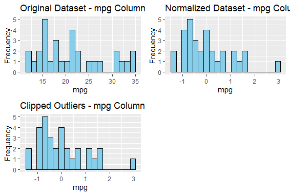
Coping with Missing, Invalid and Duplicate Data in R

This grid histogram represents the comparison between the datasets before coping with the invalid issues in our points.

Alternative sequence of transformations

[1] "Dataset after Alternative Sequence of Transformations:"
 mpg        cyl        disp          hp        drat
Mazda RX4                     NA -0.1049878 -0.57061982 -0.55695522  0.56751369
Mazda RX4 Wag       -0.052549131 -0.1049878 -0.57061982 -0.55695522  0.56751369
Datsun 710           0.173007908 -1.2248578 -0.99018209          NA  0.47399959
Hornet 4 Drive      -0.002425345 -0.1049878  0.22009369 -0.55695522 -0.96611753
Hornet Sportabout    2.954878057  1.0148821  1.04308123  0.38533258 -0.83519779
Valiant             -0.415946583 -0.1049878 -0.04616698 -0.62943890 -1.56460776
Duster 360          -0.892122554  1.0148821  1.04308123  1.40010406 -0.72298087
Merc 240D            0.373503054 -1.2248578 -0.67793094 -1.25279852  0.17475447
Merc 230             0.173007908 -1.2248578 -0.72553512 -0.77440625  0.60491932
Merc 280             1.701783396 -0.1049878 -0.50929918 -0.36849766  0.60491932
Merc 280C           -0.453539423 -0.1049878 -0.50929918 -0.36849766  0.60491932
Merc 450SE          -0.628972675  1.0148821  0.36371309  0.45781626 -0.98482035
Merc 450SL          -0.516194156  1.0148821  0.36371309  0.45781626 -0.98482035
Merc 450SLC         -0.779344035  1.0148821  0.36371309  0.45781626 -0.98482035
Cadillac Fleetwood  -1.380829473  1.0148821  1.94675381  0.82023464 -1.24665983
Lincoln Continental -1.380829473  1.0148821  1.84993175  0.96520200 -1.11574009
Chrysler Imperial   -0.841998768  1.0148821  1.68856165  1.18265303 -0.68557523
Fiat 128             1.375978784 -1.2248578 -1.22658929 -1.19481158  0.90416444
Honda Civic          1.125359851 -1.2248578 -1.25079481 -1.39776588  2.49390411
Toyota Corolla       1.563942983 -1.2248578 -1.28790993 -1.20930832  1.16600392
Toyota Corona        0.010105602 -1.2248578 -0.89255318 -0.74541278  0.19345729...........

What is Duplicate Data?

Sometimes our dataset has similar or identical rows and columns, such type of data is known as duplicate data. Due to this, we can count the same thing twice or more times based on the number of times the value has been duplicated. This alters the output and dealing with it is important. To understand this better we will create a fictional dataset as an example. This example is based on the salary, ID, age, and name of the employee. Duplicate values in such datasets can cause serious confusion and issues.

R

# Create a sample dataset with duplicate data
example_data <- data.frame(
  ID = c(1, 2, 3, 4, 5, 1, 6, 2),
  Name = c("Alice", "Bob", "Charlie", "David", "Eve", "Alice", "Frank", "Bob"),
  Age = c(25, 30, 35, 22, 28, 25, 40, 30),
  Salary = c(50000, 60000, 70000, 45000, 55000, 50000, 80000, 60000)
)

# Display the dataset with duplicate data
print("Dataset with Duplicate Data:")
print(example_data)

Output:

[1] "Dataset with Duplicate Data:"
  ID    Name Age Salary
1  1   Alice  25  50000
2  2     Bob  30  60000
3  3 Charlie  35  70000
4  4   David  22  45000
5  5     Eve  28  55000
6  1   Alice  25  50000
7  6   Frank  40  80000
8  2     Bob  30  60000

Here column 6 is a duplicate of column 1 as well and column 8 is a duplicate of column 2 making multiple values for similar things

Identify Duplicate Data

The dataset we took here is small for example therefore identifying duplicate values was easier by going through each value but if we have a large dataset, it is not possible to go through each column and identify duplicate values. It is also time-consuming, to make this issue easier we can follow the below-mentioned code:

R

# Identify duplicate rows based on all columns
duplicates_all <- example_data[duplicated(example_data), ]

# Identify duplicate rows based on selected columns (e.g., ID and Name)
duplicates_selected <- example_data[duplicated(example_data[c("ID", "Name")]), ]

# Display duplicate rows
print("Duplicate Rows (All Columns):")
print(duplicates_all)

print("Duplicate Rows (Selected Columns):")
print(duplicates_selected)

Output:

[1] "Duplicate Rows (All Columns):"
  ID  Name Age Salary
6  1 Alice  25  50000
8  2   Bob  30  60000

[1] "Duplicate Rows (Selected Columns):"
  ID  Name Age Salary
6  1 Alice  25  50000
8  2   Bob  30  60000

This code gave us the duplicated values in our dataset.

Dealing with Duplicate Data

There are several ways of dealing with duplicate data such as Deleting such rows or Aggregation of the duplicated rows or columns. We will understand how to do it with the help of the above example of salary, ID, age, and name of employees in a company.

Deleting duplicate values

We can delete the columns or rows that are twice or more than twice in our dataset.

R

# Remove duplicate rows and create a new dataset
no_duplicates_data <- unique(example_data)

# Display the dataset after removing duplicates
print("Dataset after Removing Duplicates:")
print(no_duplicates_data)

Output:

[1] "Dataset after Removing Duplicates:"
  ID    Name Age Salary
1  1   Alice  25  50000
2  2     Bob  30  60000
3  3 Charlie  35  70000
4  4   David  22  45000
5  5     Eve  28  55000
7  6   Frank  40  80000

Aggregating Duplicate Data

We can also merge these values if these values are taken for different periods and we want to merge those two rows or columns we can follow the below code:

R

# Aggregate data by summing Salary for each unique combination of ID and Name
aggregated_data <- aggregate(Salary ~ ID + Name + Age, data = example_data, sum)

# Display the aggregated dataset
print("Aggregated Dataset:")
print(aggregated_data)

Output:

[1] "Aggregated Dataset:"
  ID    Name Age Salary
1  4   David  22  45000
2  1   Alice  25 100000
3  5     Eve  28  55000
4  2     Bob  30 120000
5  3 Charlie  35  70000
6  6   Frank  40  80000

Data Matching

This is done when we want to keep the earliest column or row or just one of the duplicated values. This keeps the most relevant value out of the multiple values. The !duplicated condition is used to keep only the first occurrence of each unique combination of columns.

R

# Keep only the first occurrence of each unique combination of ID and Name
matched_data <- example_data[!duplicated(example_data[c("ID", "Name")]), ]

# Display the dataset after matching duplicates
print("Dataset after Matching Duplicates:")
print(matched_data)

Output:

[1] "Dataset after Matching Duplicates:"
  ID    Name Age Salary
1  1   Alice  25  50000
2  2     Bob  30  60000
3  3 Charlie  35  70000
4  4   David  22  45000
5  5     Eve  28  55000
7  6   Frank  40  80000

Conclusion

In this article, we understood how to deal with missing, invalid, and duplicate data in R programming language with the help of different examples. We also visualized the original and maintained dataset to understand the difference between them.