Beta-divergence loss functions in Scikit Learn
Last Updated :
08 Jun, 2023
In this article, we will learn how to use Scikit learn for visualizing different beta divergence loss functions. We will first understand what are beta divergence loss functions and then we will look into its implementation in Python using _beta_divergence function of sklearn.decomposition._nmf library in scikit learn library.
Beta Divergence Loss Function
Beta-divergence loss functions are a type of loss function used to measure the difference between two probability distributions. The divergence is measured by comparing points from the two distributions. This distance can be used to optimize the matching of distributions and determine the best fitting model. This is useful for tasks such as unsupervised learning, where probability distributions are used to represent data. Beta-divergence is related to other loss functions such as Kullback-Leibler divergence and Total Variational Distance.
The beta-divergence loss function are commonly used in non-negative matrix factorization (NMF). In NMF, the goal is to factorize a non-negative matrix into two lower-rank non-negative matrices, typically referred to as the basis matrix and the coefficient matrix. The beta-divergence loss function is used as an objective function to optimize the factorization process by minimizing the discrepancy between the target matrix and the reconstructed matrix. These functions are preferred because they are more flexible that any other loss functions for NMF and they can be used on data that is not perfectly non-negative and has a wide range of values.
Some of the use cases of these loss functions involves in clustering, anomaly detection, image segmentation, natural language processing, time series analysis, and recommendation systems.
The formula for beta-divergence loss can be expressed as:
![D_{\beta}(X|Y) \overset{\bigtriangleup}{=}\begin{cases} \frac{1}{\beta(\beta - 1)} \left[ \sum_{i=1}^{n} x_i^{\beta} - \beta \sum_{i=1}^{n} x_i y_i^{\beta - 1} + (\beta - 1) \sum_{i=1}^{n} y_i^{\beta} \right] & \text{ if } \beta \epsilon \mathbb{R}\ \{0,1\}\\ \sum_{i=1}^{n} x_{i} \log \left( \frac{x_{i}}{y_{i}} \right) & \text{ if } \beta=1 \\ \sum_{i=1}^{n} \left( \frac{x_i}{y_i} \right) - \sum_{i=1}^{n} \log \left( \frac{x_i}{y_i} \right) & \text{ if } \beta=0 \end{cases}](https://www.geeksforgeeks.org/wp-content/ql-cache/quicklatex.com-cf9cd82b8d322d66b69bb44ea3eb3067_l3.png "Rendered by QuickLaTeX.com")
where,
- X and Y are the matrices.
 and
and  are the elements of X and Y
 is the hyperparameter that controls the degree of divergence.
Beta-divergence is a generalization of other divergence measures such as the Kullback-Leibler (KL) divergence and the Total Variation (TV) distance. The specific form of the beta-divergence depends on the choice of a parameter, typically denoted as β. When β is set to 1, it corresponds to the KL divergence, and when β tends to infinity, it approximates the TV distance.
Based on different values of we can get different beta divergence loss functions. Some of the popular beta-divergence loss functions are:
- Itakura-Saito divergence: This is the divergence function with
 . This is defined as
- Kullback-Leibler divergence: This is the divergence function with
 . This divergence is used to measure the difference between two probability distributions. It is defined as
  .
. - Frobenius norm: This is the divergence function with
 . This basically calculates the distance between two matrices (mean-squared error). It is defined as
The beta divergence loss function that is best for a particular application will depend on the characteristics of the data. In general, the Frobenius norm loss function is a good choice for data that is perfectly non-negative. The Kullback-Leibler divergence is a good choice for data that is not perfectly non-negative. The Itakura-Saito divergence is a good choice for data that has a wide range of values.
Code Implementation
To implement this we will first import the required libraries.
Python3
import numpy as np
import matplotlib.pyplot as plt
from sklearn.decomposition._nmf import _beta_divergence
|
Now, we will plot and compare different Beta-divergence loss functions.
Python3
x = np.linspace(0, 5, 100)
y = np.zeros(x.shape)
beta_loss = ['Itakura-Saito', 'Kullback-Leibler', 'Frobenius norm']
beta = [0.0, 1.0, 2.0]
for j, beta in enumerate(beta):
for i, xi in enumerate(x):
y[i] = _beta_divergence(1, xi, 1, beta)
name = f'beta = {beta}: {beta_loss[j]}'
plt.plot(x, y, label=name)
plt.xlabel("x")
plt.ylabel("D(1, x)")
plt.title("Beta-Divergence(1, x)")
plt.legend(loc='upper center')
plt.grid(True)
plt.axis([0, 4, 0, 3])
plt.show()
|
Output:
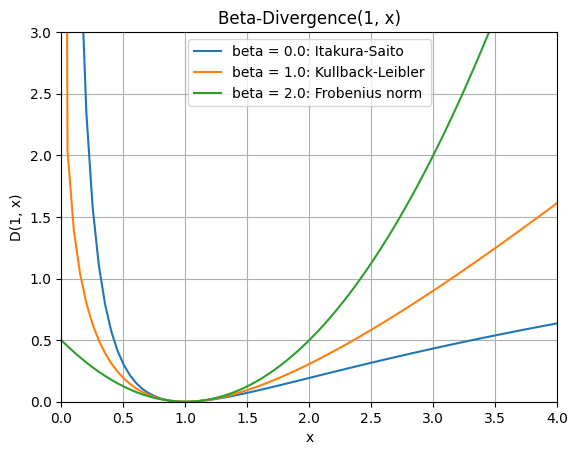
Comparing different beta divergence loss functions
Share your thoughts in the comments
Please Login to comment...