Affinity Propagation

Affinity Propagation is a clustering algorithm that is commonly used in Machine Learning and data analysis. Unlike other traditional clustering algorithms which require specifying the number of clusters beforehand, Affinity Propagation discovers cluster centres and assigns data points to clusters autonomously. It is particularly useful when the number of clusters is not known in advance or when the data doesn’t conform to spherical or convex cluster shapes. In this article, we will discuss about Affinity propagation, its parameters and implementation with evaluation.

What is Affinity Propagation?

Affinity Propagation is based on the concept of “message-passing” between data points to identify cluster centres and assign data points to these centres automatically. It utilizes “exemplars,” which are typical data points representing other data points within the same cluster. The objective of the algorithm is to identify the most representative exemplars of the overall data and employ them to cluster the data into compatible groups. This algorithm is especially suitable for data with numerous clusters or data exhibiting intricate, non-linear distribution patterns.

The core of the algorithm is represented by three matrices which are Similarity Matrix(S), Responsibility Matrix (R) and Availability Matrix (A).

1. Similarity Matrix(S): To determine the similarity between data points, we calculate a ‘similarity score’ based on their features, rather than their visual attributes like colour and size. The ‘similarity score’ is computed using the negative squared distance between the data points. This involves taking the distance between the points, squaring it, and then making the result negative. The resulting matrix of similarity scores for every pair of data points is called the ‘similarity matrix’ (S). For every pair of data points i and k, we calculate:
   
   where, is the squared Euclidean distance between the two points.
2. Responsibility Matrix(R): The matrix used to represent the suitability of one data point to be the exemplar (cluster centre) for another data point. R(i, k) is a value that indicates how well data point ‘i’ is suited to be the exemplar for data point ‘k’. The update process of each iteration for this matrix is:
   
   similarity(i, k) represents the similarity or affinity between data point ‘i’ and data point ‘k’. The responsibility r(i, k) is updated by subtracting this maximum sum from the similarity(i, k).
3. Availability Matrix (A): The availability matrix is used to represent the “availability” of each data point to serve as an exemplar for other data points. The calculation reflects the competition between different data points to serve as exemplars and helps in determining the most suitable exemplars for the clusters.
   
   Where a(i, k) calculates the availability value for a specific data point i and a potential exemplar k.
   1. The term r(k, k) represents the “responsibility” of the potential exemplar k to itself, and the term max{0, r(i’, k)} for all i’≠i, k represents the “responsibility” of other data points i’ to the potential exemplar k.
   2. The availability value a(i, k) is then calculated as the minimum of 0 and the sum of r(k, k) and the maximum of 0 and the responsibilities of other data points to the potential exemplar k.
   3. r(k, k) represents the responsibility of data point ‘k’ to be its own exemplar. The term max{0, r(i’, k)} calculates the maximum value between 0.

The equations are iteratively applied until convergence, meaning that until the values in matrices stabilize. Once convergence is reached, cluster assignments can be derived from the final matrices R and A.

Key-steps of Affinity propagation

Affinity Propagation clustering algorithm has several step which are discussed below

1. Similarity Computation: This algorithm first calculates a similarity (or dissimilarity) matrix which quantifies the similarity between pairs of data points. The choice of similarity metric depends on the data and the problem what we’re working on. There are some common metrics like Euclidean distance, negative squared Euclidean distance etc.
2. Responsibility Update: Then this algorithm initializes the responsibility matrix (R), where R(i, k) represents the responsibility of data point i to be the exemplar for data point k. We have already discussed about it previously in this article. Here data points compete to be exemplars based on their similarity and the responsibility which they receive from other data points.
3. Availability Update: Then it initializes the availability matrix (A), where A(i, k) represents the availability of data point k to choose data point i as its exemplar. This step is also already discussed in this article. Here data points consider the availability of other data points to be their exemplars. If a data point has high availability from other data points then it is more likely to be chosen as an exemplar.
4. Update Responsibility and Availability: Then it updates the responsibility and availability matrices iteratively until convergence which is reached when the matrices no longer change significantly between iterations.
5. Net Responsibility Calculation: Then it calculates the net responsibility for each data point by summing its responsibility and availability.
6. Exemplar Selection: Then a crucial task is to identify exemplars as data points with high net responsibility. These exemplars represent the cluster centers.
7. Cluster Assignment: Finally it assigns each data point to the nearest exemplar (based on similarity) to form clusters.

Working Principals of Affinity Propagation

The algorithm begins by initializing the “responsibility” and “availability” matrices to zero.

Similarity Matrix: All similarities between data points are represented in a similarity matrix. This matrix does not need to contain all the similarity values to ensure a reasonable number of clusters.

Message Passing: Each data point is treated as a potential exemplar. Real-valued messages are exchanged between data points until a high-quality set of exemplars and corresponding clusters gradually emerges. The algorithm involves passing two kinds of messages:

• Responsibility Messages: These messages are sent from data point i to candidate exemplar k and reflect the accumulated evidence for how well-suited point k is to serve as the exemplar for point i, taking into account other potential exemplars for point i.
• Availability Messages: These messages are sent from candidate exemplar k to point i and reflect the accumulated evidence for how appropriate it would be for point i to choose point k as its exemplar, taking into account the support from other points that point k should be an exemplar.

Convergence: The algorithm iteratively updates the responsibility and availability matrices until a stopping criterion is met. This could be a predefined number of iterations or until the algorithm converges.

Exemplars and Clusters: At the end of the process, the algorithm provides a set of exemplars and the assignment of all other data points to these exemplars, effectively partitioning the data into clusters.

The steps are implemented in the algorithm to iteratively find the best exemplars and form clusters around them.

Benefits of using Affinity Propagation

Using Affinity Propagation for clustering has several benefits which are listed below:

1. Automatic Cluster Center Detection: Affinity Propagation automatically identifies cluster centers and total number of clusters which makes it suitable for datasets with an unknown or variable number of clusters and useful for large complex real-world datasets.
2. Robust to Noise and Outliers: Affinity Propagation is relatively robust to noise and outliers in the data which makes it useful in various applications like image segmentation, document clustering and biological dataset analysis etc.
3. Handles Non-Spherical Clusters: Unlike some traditional clustering algorithms, Affinity Propagation can handle clusters of various shapes and sizes.
4. Scalability: It can be applied to large datasets, although it may require optimization for computational efficiency.

Affinity Propagation Step-by-step implementation

Importing required libraries

At first, we will import all required Python libraries like NumPy, Matplotlib, Seaborn, Pandas and SKlearn etc.

Python3

import pandas as pd
import numpy as np
import matplotlib.pyplot as plt
from sklearn.cluster import AffinityPropagation
from sklearn import metrics
from sklearn.preprocessing import StandardScaler
from sklearn.decomposition import PCA
import seaborn as sns

Dataset loading and pre-processing

Now we load the dataset for clustering. After that, we will use to Standard Scaler to prepare the dataset for Affinity propagation.

Python3

# Load the Mall Customer Segmentation dataset and drop any NaN values and irrelavent columns
data = pd.read_csv('Mall_Customers.csv').dropna().drop('CustomerID', axis=1)
# Select relevant features for clustering
features = ['Annual Income (k$)', 'Spending Score (1-100)']
X = data[features]
# Standardize the data
scaler = StandardScaler()
X_std = scaler.fit_transform(X)

Exploratory Data Analysis

Exploratory Data Analysis(EDA) helps us to gain deeper insights about the dataset which is very crucial in clustering algorithm implementation.

• Correlation matrix: Visualizing correlation matrix will help us to understand how the features are correlated to each other. From here we can understand that only which features can be chosen for clustering.

Python3

# EDA 1: Correlation Matrix
correlation_matrix = data.corr(numeric_only=True)
plt.figure(figsize=(7, 7))
sns.heatmap(correlation_matrix, annot=True, cmap="coolwarm", fmt=".2f")
plt.title("Correlation Matrix")
plt.show()

Output:

Correlation Matrix

So, from it we can see that we can only select these three features. And as you can see we have only selected two features in our code of Data loading subsection.

Pairwise Feature Scatter Plots is a very useful EDA for clustering. It provides a grid of scatter plots and histograms that visualize relationships between pairs of features in our dataset which is a valuable tool for understanding the distribution and interaction of variables as in a single plot we can visualize distribution of features, pairwise relationships between features and density estimation.

Python3

# EDA 2: Pairplot
sns.pairplot(data, palette="Set1", hue="Gender", diag_kind="kde", height=2)
plt.suptitle("Pairwise Feature Scatter Plots", y=1.02)
plt.show()

Output:

Pair-wise feature distribution plot

Affinity Propagation Clustering and performance evaluation

Now we will employ Affinity Propagation by specifying required parameters of it which are discussed below:

1. Preference: The preference parameter plays an important role and represents the input that indicates how likely a data point is to be chosen as an exemplar. It influences the number of clusters that will be formed and the data points that will be assigned as exemplars
2. max_iter: This parameter determines the maximum number of iterations (passes over the data) which will be performed by the Affinity Propagation algorithm before terminating. The default value is 200 but here we have used higher value which is better for convergence.
3. convergence_iter: This parameter controls the number of iterations with no change in the cluster assignments which must occur for the algorithm to consider the solution as converged. We have set it to 16 which means the algorithm will continue iterating until it finds a solution where the cluster assignments do not change for 16 consecutive iterations, indicating convergence.
4. random_state: This parameter handles the randomness which ensures the initialization of cluster centers and the order of processing data points remains same between different runs.
5. damping: It controls the convergence speed of the algorithm which it set to 0.9(close to 1) means that algorithm converges more slowly. This is used for more stable and accurate cluster assignments.

Preference parameter impact on Affinity Propagation Clustering

The code creates a line plot to visualize the relationship between preference values and silhouette scores, aiding in the selection of an optimal preference parameter for clustering.

Python

Preference = [-50, -40, -30,-20, -10]
silhouette_scores = []
for preference in Preference:
    model = AffinityPropagation(preference=preference, random_state=42)
    model.fit(X_std)

    silhouette_scores.append(metrics.silhouette_score(X_std , model.labels_))
silhouette_scores

# Create line plot of `Preference` vs `silhouette_scores`
plt.plot(Preference , silhouette_scores )
plt.grid()
plt.show()

Output:

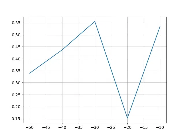
Preference vs silhouette_scores

Here, -30, resulting in higher value of preference parameter is the optimal preference.

Apply Affinity Propagation Clustering

Python

af = AffinityPropagation(preference= -30, max_iter=50, damping=0.7, random_state=42, convergence_iter=20).fit(X_std)

# Predict cluster labels
cluster_labels = af.labels_
cluster_labels

Output:

array([0, 1, 0, 1, 0, 1, 0, 1, 0, 1, 0, 1, 0, 1, 0, 1, 0, 1, 0, 1, 0, 1,
       0, 1, 0, 1, 0, 1, 0, 1, 0, 1, 0, 1, 0, 1, 0, 1, 0, 1, 2, 1, 2, 2,
       0, 1, 2, 2, 2, 2, 2, 2, 2, 2, 2, 2, 2, 2, 2, 2, 2, 2, 2, 2, 2, 2,
       2, 2, 2, 2, 2, 2, 2, 2, 2, 2, 2, 2, 2, 2, 2, 2, 2, 2, 2, 2, 2, 2,
       2, 2, 2, 2, 2, 2, 2, 2, 2, 2, 2, 2, 2, 2, 2, 2, 2, 2, 2, 2, 2, 2,
       2, 2, 2, 2, 2, 2, 2, 2, 2, 2, 2, 2, 2, 4, 3, 4, 3, 4, 3, 4, 3, 4,
       3, 4, 3, 4, 3, 4, 3, 4, 3, 4, 3, 4, 3, 4, 3, 4, 3, 4, 3, 4, 3, 4,
       3, 4, 3, 4, 3, 4, 3, 4, 3, 4, 3, 4, 3, 4, 3, 4, 3, 4, 3, 4, 3, 4,
       3, 4, 3, 4, 3, 4, 3, 4, 3, 4, 3, 4, 3, 4, 3, 4, 3, 4, 3, 4, 3, 4,
       3, 4])

After that, we will evaluate its performance using Silhouette Score.

Python3

silhouette_score = metrics.silhouette_score(X_std, cluster_labels)
print(f"Silhouette Score: {silhouette_score}")

Output:

Silhouette Score: 0.5529643053885619

Silhouette Score of 0.5529 represents a reasonably good degree of separation between the clusters. The Silhouette score is >0 which depicts that the algorithm has created clusters well and no overlap encountered(score 0).

Visualizing Clusters

Now it is time visualize the clusters. We will create a plot where clustering effect can be visualized.

Python3

# Reduce dimensionality to 2D for visualization
pca = PCA(n_components=2)
X_r = pca.fit_transform(X_std)

# Scatter plot the data points with different colors for each cluster
unique_clusters = np.unique(cluster_labels)
colors = plt.cm.tab20(unique_clusters)
lw = 2

for cluster_id, color in zip(unique_clusters, colors):
    plt.scatter(X_r[cluster_labels == cluster_id, 0], X_r[cluster_labels == cluster_id, 1],
                color=color, alpha=0.8, lw=lw, label=f'Cluster {cluster_id}')

plt.legend(loc='best', shadow=False, scatterpoints=1, title='Clusters')
plt.title('Affinity Propagation Clustering of Mall Customers')
plt.xlabel('PCA Dimension 1')
plt.ylabel('PCA Dimension 2')

plt.show()

Output:

Effect of Affinity Propagation

Conclusion

We can conclude that using Affinity Propagation is an efficient way to make clusters for real-world complex and large datasets. Our results shows that it performed well in the dataset but there is still some spaces for parameter tuning.