What is Monte Carlo (MC) dropout?

Monte Carlo Dropout was introduced in a 2016 research paper by Yarin Gal and Zoubin Ghahramani, is a technique that combines two powerful concepts in machine learning: Monte Carlo methods and dropout regularization. This innovation can be thought of as an upgrade to traditional dropout, offering the potential for significantly more accurate predictions. It is done is at time of testing . In this article, we’ll delve into the concepts and workings of Monte Carlo Dropout.

Understanding Dropout

Dropout is primarily used as a regularization technique, a method employed to fine-tune machine learning models. It aims to optimize the adjusted loss function while avoiding the issues of overfitting or underfitting. When implemented, traditional dropout typically results in a modest increase in model accuracy, usually in the range of 1% to 2%. This improvement is credited to its effectiveness in reducing overfitting, which, in turn, minimizes errors in the model’s predictions.

The dropout rate typically falls within the range of 0 (signifying no dropout) to 0.5 (meaning around 50% of all neurons will be deactivated). The specific value is determined by factors such as the type of network, the size of its layers, and the extent to which the network tends to overfit the training data. At every iteration different set of neurons are dropped, corresponding with its ingoing and outgoing directions.

Monte Carlo Dropout

The Monte Carlo Dropout technique, as introduced by Gal and Ghahramani in 2016, involves estimation of uncertainty in predictions made by models. By applying dropout at test time and running multiple forward passes with different dropout masks, the model produces a distribution of predictions rather than a single point estimate. This distribution provides insights into the model’s uncertainty about its predictions, effectively regularizing the network.

Step 1: Estimation of Predictive Distribution

It leverages the principles of Bayesian neural networks to estimate uncertainty and improve the predictive capabilities of neural network models. One of the primary goals of Monte Carlo Dropout is to obtain a predictive distribution, which allows for the uncovering of uncertainty in the model’s predictions. The predictive distribution is a probability distribution that represents the uncertainty about the value of a future observation or outcome given the data, observed.

To achieve this, Monte Carlo Dropout employs the concept of learning a distribution over functions, or equivalently, a distribution over the parameters, known as the parametric posterior distribution. This distribution captures the uncertainty in the model’s parameters and enables the exploration of different network configurations.

Where, represents dropout mask, sampled from approximate parametric posterior.

Step 2: Exploration of Diverse Network Configurations

Each dropout configuration corresponds to a different sample from the approximate parametric posterior distribution. This process allows for the exploration of diverse network configurations and facilitates the learning of a predictive distribution.

Step 3: Monte Carlo Integration for Uncovering Predictive Distribution

By sampling from the approximate posterior distribution, Monte Carlo Dropout enables Monte Carlo integration of the model’s likelihood, leading to the uncovering of the predictive distribution. This predictive distribution provides insights into the uncertainty associated with the model’s predictions, allowing for more informed decision-making.

However, the likelihood may be assumed to be Gaussian distributed for simplicity.

The Gaussian function, denoted by is characterized by the mean and variance parameters, which are obtained from simulations using the Monte Carlo dropout Bayesian neural network (BNN).

Step 4: Estimation of Uncertainty and Reliable Predictions

This approach allows for the estimation of uncertainty and the generation of more reliable predictions, making the model more robust and dependable.

Applying Dropout During Testing-Monte Carlo

The process of Monte Carlo Dropout during testing involves two key steps:

1.For predicating test data we’ll keep drop out data activated : For predicting test data, we keep dropout in effect. This means that different sets of neurons are deactivated at each iteration.

Model(x_test,Training=True)

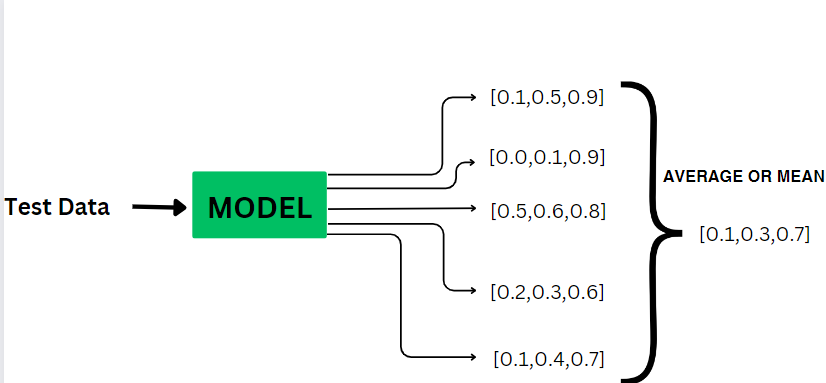
2.Perform any simulation to find ‘T’ output for test data :For every test data that we are passing through the model we’ll try to get some T results i.e. T specifies my simulation . Each dropout model provides different scores, and then we compute the average of these scores. The final prediction is the average of predictions from .

Mathematically,

In the equation:

T represents the number of forward passes or samples we take with different dropout masks. Each forward pass generates a prediction, denoted as .

Dropout masks refer to the random patterns of dropout applied to the neurons in a neural network during each forward pass. By using different dropout masks for each forward pass, the network is forced to learn more robust representations that are not overly dependent on specific neurons. This helps improve the generalization ability of the network and reduces the risk of overfitting. The sum of all the predictions, , represents the cumulative output of the network across all the forward passes.The term () is a scaling factor that ensures the final prediction is an average of the individual predictions. It divides the sum of the predictions by the total number of forward passes, T.

The final prediction, y_final, represents the average of the T predictions and can be interpreted as the expected value or mean prediction of the network. It provides a more reliablе estimate compared to a single prediction obtained without dropout.

Building and testing the model without Monte Carlo Dropout Method

Step 1: Import the necessary libraries

Python

import numpy as np
import pandas as pd
import tensorflow as tf
from tensorflow import keras
from sklearn.datasets import load_iris
from sklearn.model_selection import train_test_split

Step 2: Load and split the Dataset

Python

data = load_iris()
df = pd.DataFrame(data.data, columns=data.feature_names)
df['target'] = data.target
X = df.iloc[:, :-1]
y = df['target']
X_train, X_test, y_train, y_test = train_test_split(X, y, test_size=0.2, random_state=42)

Step 3: Create a neural network with dropout layers

Python

model = keras.Sequential([
    keras.layers.Input(shape=(4,)),
    keras.layers.Dense(64, activation='relu'),
    keras.layers.Dropout(0.5),
    keras.layers.Dense(32, activation='relu'),
    keras.layers.Dropout(0.5),
    keras.layers.Dense(3, activation='softmax')
])
# Compile the model
model.compile(optimizer='adam', loss='sparse_categorical_crossentropy', metrics=['accuracy'])

model.fit(X_train, y_train, epochs=50, verbose=0) # training the model

Step 4:Evaluate the model

Python

standard_accuracy = model.evaluate(X_test, y_test, verbose=0)[1]
print(f"Standard Model Accuracy: {standard_accuracy}")

Output:

Standard Model Accuracy: 0.7666666507720947

Building and testing the model with Monte Carlo Dropout Method

Step 1: Training a Model with Monte Carlo Dropout

The model is being trained for one epoch at a time for a total of 50 epochs. After each epoch, Monte Carlo dropout predictions are generated for the test data using the trained model, with 100 Monte Carlo samples used to estimate the average predictions and uncertainty to obtain the final prediction and computes the uncertainty as the variance of the predictions across the samples.

Python

# MONTE CARLO DROPOUT
n_samples = 100

def monte_carlo_dropout_predict(model, X, n_samples):
    predictions = []
    for _ in range(n_samples):
        predictions.append(model(X, training=True))

    predictions = np.array(predictions)
    mean_predictions = predictions.mean(axis=0)
    uncertainty = predictions.var(axis=0)

    return mean_predictions, uncertainty
X_test=np.array(X_test) # to convert tuple to array format

Step 2: Evaluate the model

The code calculates the accuracy of the model’s predictions with Monte Carlo dropout by comparing the maximum of the average predictions with the true labels and taking the mean of the resulting boolean array to get the proportion of correct predictions.

Python

accuracy = np.mean(np.argmax(mean_predictions, axis=1) == y_test)
print(f"Epoch {_+1}, Accuracy with Monte Carlo Dropout: {accuracy}")

Output:

Accuracy with Monte Carlo Dropout: 0.8666666666666667

The process is repeated for 50 epochs. An accuracy of 86% with Monte Carlo Dropout suggests that the model is performing well on the given task and has correctly predicted the training samples. Clearly, Monte Carlo Dropout has more accuracy then traditional Dropout.

Monte Carlo Dropout offers several advantages

• Uncertainty Estimation: It provides a measure of uncertainty for model predictions, which can be crucial for applications such as medical diagnosis, autonomous vehicles, and financial forecasting.
• Robustness: The technique makes predictions more robust by capturing the inherent uncertainty in real-world data. It helps the model recognize when it’s uncertain and refrain from making unreliable predictions.
• Model Calibration: Monte Carlo Dropout can be used to calibrate models, ensuring that the predicted probabilities align with actual outcomes.
• Bayesian Neural Networks: In a broader context, Monte Carlo Dropout can be seen as a simple way to turn a standard neural network into a Bayesian neural network, which models the uncertainty in its predictions more explicitly.

” Monte Carlo Dropout is an advanced deep learning technique that enhances model accuracy by simulating multiple iterations of dropout during testing, producing more reliable predictions through probabilistic reasoning. “

Conclusion

In conclusion, Monte Carlo Dropout is an innovative technique that combines Monte Carlo methods and dropout regularization to improve the accuracy and reliability of machine learning models. By simulating multiple iterations of dropout during testing, it provides uncertainty estimation, enhances model robustness, and enables model calibration. This advanced technique offers a more accurate and probabilistic approach to prediction, making it a valuable tool in various domains.