Optical Character Recognition using TensorFlow

Optical Character Recognition (OCR) stands as a transformative force, bridging the gap between the physical and digital worlds. OCR enables machines to interpret and convert printed or handwritten text into machine-readable data, revolutionizing how we interact with information. This article explores the powerful capabilities of OCR and presents a TensorFlow-based model, a testament to the evolution of deep learning in unlocking the potential of visual data.

What is Optical Character Recognition(OCR)?

Optical Character Recognition (OCR) is a technology that empowers computers to recognize and interpret text from images, whether scanned documents, photos, or handwritten notes. It has emerged as a vital component in various fields, from document digitization to aiding visually impaired individuals. The primary goal of OCR is to convert visual representations of characters into editable and searchable data, making it an invaluable tool in our increasingly digitized society. As we delve into the capabilities of OCR, we’ll showcase a practical implementation using TensorFlow, a popular open-source machine learning framework.

Optical Character Recognition(OCR) Implementation using TensorFlow

Before starting the implementation, let’s install TensorFlow using the following command:

!pip install tensorflow

TensorFlow is an open-source machine learning library developed by the Google Brain team. We will be using TensorFlow for implementing OCR as TensorFlow provides a flexible and extensive framework to build customized OCR models.

Importing Libraries

For the implementation, we will be using open cv, numpy, matplotlib, tensorflow, and keras.

Python3

import tensorflow as tf
from keras.models import Sequential
from keras.layers import Conv2D, Flatten, MaxPooling2D, Dense
import os
import cv2
import numpy as np

Loading dataset and Preprocessing

You can download the dataset from here and unzip the folder using following command:

!unzip /content/OCR_dataset.zip

Reading and Preprocessing Images:

• files = os.path.join(dir, j) creates the full path to the current image file.
• img = cv2.imread(files) reads the image using OpenCV.
• img = cv2.resize(img, (64,64)) resizes the image to a fixed size (64×64 pixels).
• img = np.array(img, dtype=np.float32) converts the image to a NumPy array with float32 data type.
• img = img/255 normalizes the pixel values to the range [0, 1].

Building Lists of Images and Labels:

• images.append(img) adds the preprocessed image to the list images.
• labels.append(i) adds the corresponding label (class) to the list labels. The label is determined by the subdirectory name.

Python3

images = []
labels = []

path = '/content/data/training_data'

dir_list = os.listdir(path)
for i in dir_list:
  dir = os.path.join(path, i)
  file_list = os.listdir(dir)
  for j in file_list:
    files = os.path.join(dir, j)
    img = cv2.imread(files)
    img = cv2.resize(img, (64,64))
    img = np.array(img, dtype=np.float32)
    img = img/255
    images.append(img)
    labels.append(i)

Converting list to NumPy arrays:

• ‘X’ is a NumPy array containing the preprocessed images. Each element of X is a 3D array representing an image.
• ‘y’ is a NumPy array containing the corresponding labels for each image.

Python3

X = np.array(images)
y = np.array(labels)

Label Encoding:

The fit_transform method of the LabelEncoder class is used to fit the encoder to the unique labels in y and transform them into numerical values.

Python3

from sklearn.preprocessing import LabelEncoder
le = LabelEncoder()
y = le.fit_transform(y)

Shuffling the data:

• The shuffle function is used to shuffle the order of samples and their corresponding labels.
• X_sh contains the shuffled images.
• y_sh contains the corresponding shuffled labels.
• The random_state=42 argument ensures reproducibility by initializing the random number generator with a specific seed.
• This is done to introduce randomness in the data which is useful while training.

Python3

from sklearn.utils import shuffle
X_sh, y_sh = shuffle(X, y, random_state=42)

Building the Model

The model is implemented using the Keras API with a TensorFlow backend.

The model architecture consists of the following layers:

• Convolutional layer with 16 filters, a 3×3 kernel, and ReLU activation.
• Max pooling layer to reduce spatial dimensions.
• Convolutional layer with 32 filters and ReLU activation.
• Max pooling layer.
• Convolutional layer with 64 filters and ReLU activation.
• Max pooling layer.
• Convolutional layer with 128 filters and ReLU activation.
• Max pooling layer.
• Flatten layer to prepare for fully connected layers.
• Dense (fully connected) layer with 128 neurons and ReLU activation.
• Dense layer with 64 neurons and ReLU activation.
• Dense output layer with 36 neurons and softmax activation for multiclass classification.

Python3

model = Sequential()
model.add(Conv2D(filters=16, kernel_size=(3,3), activation='relu', input_shape=(64,64,3)))
model.add(MaxPooling2D())
model.add(Conv2D(filters=32, kernel_size=(3,3),  activation='relu'))
model.add(MaxPooling2D())
model.add(Conv2D(filters=64, kernel_size=(3,3),  activation='relu'))
model.add(MaxPooling2D())
model.add(Conv2D(filters=128, kernel_size=(3,3), activation='relu'))
model.add(Flatten())
model.add(Dense(units=128, activation='relu'))
model.add(Dense(units=64, activation='relu'))
model.add(Dense(units=36, activation='softmax'))

Model compiling and training

Compiling the Model:

• optimizer=’adam’: Adam optimization algorithm is chosen for adaptive learning rates.
• loss=’sparse_categorical_crossentropy’: Loss function for multi-class classification with integer labels.
• metrics=[‘accuracy’]: Monitoring accuracy during training.

Training the Model:

• model.fit(X_sh, y_sh, validation_split=0.2, batch_size=16, epochs=10)
• X_sh and y_sh are shuffled and preprocessed images and labels.
• validation_split=0.2: 20% of the training data used for validation.
• batch_size=16: Number of samples in each training iteration.
• epochs=10: Number of passes through the entire training dataset.

Python3

model.compile(optimizer='adam', loss='sparse_categorical_crossentropy', metrics = ['accuracy'])
history = model.fit(X_sh, y_sh ,validation_split=0.2, batch_size=16, epochs=10)

Output:

Epoch 1/10
1032/1032 [==============================] - 87s 79ms/step - loss: 0.7324 - accuracy: 0.7997 - val_loss: 0.2487 - val_accuracy: 0.9261
Epoch 2/10
1032/1032 [==============================] - 77s 74ms/step - loss: 0.1897 - accuracy: 0.9410 - val_loss: 0.1610 - val_accuracy: 0.9544
Epoch 3/10
1032/1032 [==============================] - 77s 75ms/step - loss: 0.1284 - accuracy: 0.9553 - val_loss: 0.1720 - val_accuracy: 0.9501
Epoch 4/10
1032/1032 [==============================] - 71s 69ms/step - loss: 0.1075 - accuracy: 0.9615 - val_loss: 0.1377 - val_accuracy: 0.9617
Epoch 5/10
1032/1032 [==============================] - 71s 69ms/step - loss: 0.0870 - accuracy: 0.9699 - val_loss: 0.1620 - val_accuracy: 0.9542
Epoch 6/10
1032/1032 [==============================] - 70s 68ms/step - loss: 0.0777 - accuracy: 0.9714 - val_loss: 0.1518 - val_accuracy: 0.9615
Epoch 7/10
1032/1032 [==============================] - 70s 68ms/step - loss: 0.0656 - accuracy: 0.9752 - val_loss: 0.1838 - val_accuracy: 0.9627
Epoch 8/10
1032/1032 [==============================] - 69s 67ms/step - loss: 0.0595 - accuracy: 0.9771 - val_loss: 0.1525 - val_accuracy: 0.9603
Epoch 9/10
1032/1032 [==============================] - 69s 67ms/step - loss: 0.0580 - accuracy: 0.9778 - val_loss: 0.1965 - val_accuracy: 0.9595
Epoch 10/10
1032/1032 [==============================] - 70s 68ms/step - loss: 0.0524 - accuracy: 0.9793 - val_loss: 0.1378 - val_accuracy: 0.9629

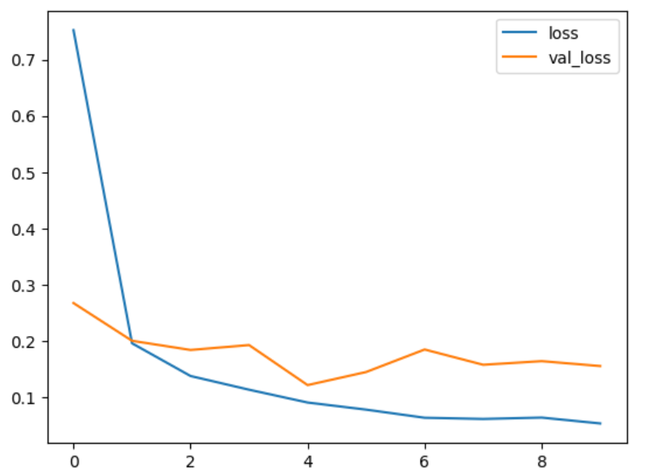
The training history, including loss and accuracy metrics on both training and validation sets, is stored in the history variable for later analysis.

Python3

plt.plot(history.history['loss'])
plt.plot(history.history['val_loss'])
plt.legend(['loss', 'val_loss'])

Output:

Model Testing

We do similar preprocessing steps taken for the training dataset.

Python3

test_images = []
test_labels = []

path = '/content/data/testing_data'

dir_list = os.listdir(path)
for i in dir_list:
  dir = os.path.join(path, i)
  file_list = os.listdir(dir)
  for j in file_list:
    files = os.path.join(dir, j)
    img = cv2.imread(files)
    img = cv2.resize(img, (64,64))
    img = np.array(img, dtype=np.float32)
    img = img/255
    test_images.append(img)
    test_labels.append(i)

Python3

X_test = np.array(test_images)
y_test = np.array(test_labels)

Making predictions

• preds = model.predict(X_test): Using the trained model to make predictions on the test dataset (X_test).
• np.argmax(preds, axis=1): Obtaining the index of the class with the highest predicted probability for each sample.
• le.inverse_transform(…): Inverse transforming the predicted indices back to the original class labels using the LabelEncoder (le).

Python3

preds = model.predict(X_test)
predicted_labels = le.inverse_transform(np.argmax(preds, axis=1))

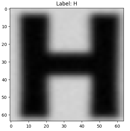
Visualize the predictions

Python3

plt.imshow(X_test[197])
plt.title(f"Label: {predicted_labels[197]}")
plt.show()

Output:

Model Evaluation

Label Encoding for Test Data:

• y_test = le.fit_transform(y_test): Applying label encoding to the true labels (y_test) of the test dataset using the same LabelEncoder (le) used during training.

Evaluating the Model on Test Data:

• test_loss, test_accuracy = model.evaluate(X_test, y_test): Evaluating the trained model on the test dataset.
• X_test: Test images.
• y_test: True labels for the test dataset.
• test_loss: The loss computed on the test dataset.
• test_accuracy: The accuracy of the model on the test dataset.

Printing Test Accuracy:

• print(f”Test Accuracy: {test_accuracy}”): Displays the test accuracy achieved by the model on the test dataset.

Python3

y_test = le.fit_transform(y_test)
test_loss, test_accuracy = model.evaluate(X_test, y_test)
print(f"Test Accuracy: {test_accuracy}")

Output:

Test Accuracy: 0.9811508059501648

We can conclude that the model has a very high accuracy of 98.61% and performs well on unseen data too.

Applications of Optical Character Recognition

• Document Digitization: OCR plays a pivotal role in converting paper-based documents into digital formats, facilitating efficient storage, retrieval, and search functionalities. Businesses can streamline their operations by digitizing vast archives of paperwork.
• Automated Data Entry: OCR automates the extraction of information from invoices, receipts, and forms, reducing manual data entry efforts. This not only improves accuracy but also enhances productivity in data-intensive tasks.
• Text Extraction from Images: OCR is widely used to extract text content from images, enabling the analysis of textual information present in photographs or screenshots. This finds applications in augmented reality, image indexing, and more.
• Accessibility for Visually Impaired: OCR technology contributes to making digital content accessible to visually impaired individuals. By converting text from images into speech or braille, OCR aids in creating an inclusive digital environment.
• Language Translation: OCR can be integrated with language translation tools, allowing users to translate text from images or scanned documents. This is valuable for breaking down language barriers in diverse settings.

Conclusion

The article explored OCR and showcased a practical implementation using Tensorflow. The Tensorflow-based OCR model demonstrated the key steps in implementing OCR, including dataset loading, image preprocessing, model building, training, and evaluation. The model achieved a remarkable accuracy of 98.61% on the test dataset, showcasing its effectiveness in recognizing characters from diverse images.