Flight Fare Prediction Using Machine Learning

In this article, we will develop a predictive machine learning model that can effectively predict flight fares.

Why do we need to predict flight fares?

There are several use cases of flight fare prediction, which are discussed below:

1. Trip planning apps: Several Travel planning apps use airfare calculators to help users find the best time to book flights. Through fare trends, these apps let users make informed decisions on when to buy tickets and get the best deals.
2. Revenue management for airlines: Airlines use airfare forecasting systems to optimize pricing strategies and maximize revenue. By analyzing historical data and market demand, airlines can dynamically adjust ticket prices to reflect changes in supply and demand, ultimately providing they get it up.
3. Corporate travel management: Companies that typically book flights for business travel rely on airfare forecasts to manage travel expenses. By anticipating future fares, corporate travel managers can negotiate better deals with airlines, better budget travel, and optimize itineraries to lower costs.
4. Travel insurers: Travel insurers include airfare forecasts in their services to cover trip cancellations. By monitoring fare fluctuations and anticipating price increases, travel insurance companies can help travellers protect their investments by offering airfare reimbursement, as unforeseen conditions may require cancellation or modification of their policies.

Step-by-step implementation in Python

Importing required libraries

At first, we will import all required Python libraries like Pandas, Matplotlib, NumPy, SKlearn etc.

Python3

# Importing necessary libraries
import pandas as pd
import numpy as np
from sklearn.model_selection import train_test_split, RandomizedSearchCV
from sklearn.ensemble import ExtraTreesRegressor, AdaBoostRegressor
from sklearn.metrics import mean_absolute_error, r2_score
import matplotlib.pyplot as plt
import seaborn as sns

Dataset loading

Now we will load a Flight Fare dataset to our runtime.

Python3

# Load the dataset
url = "https://raw.githubusercontent.com/MeshalAlamr/flight-price-prediction/main/data/NYC_SVO.csv"
df = pd.read_csv(url)

Data Pre-processing

• Now, we will perform data preprocessing tasks for the flight price prediction dataset. Firstly, we convert the ‘Duration’ column to minutes by splitting the string and calculating the total duration in minutes.
• Next, we convert the ‘Total stops’ column to numeric values by replacing categorical values with their corresponding numerical equivalents. Then, we will convert the ‘Price’ column to numeric format after removing currency symbols and commas.
• After that, we will drop unnecessary columns such as ‘Duration’, ‘Total stops’, and ‘Date’ from the dataset. Following this, we encode categorical variables using one-hot encoding to convert them into numerical format for model compatibility. Finally, we will split the dataset into features (X) and the target variable (y), and further splits the data into training and testing sets using a test size of 20%.

Python3

# Data Preprocessing
# Convert 'Duration' column to minutes
df['Duration_Minutes'] = df['Duration'].str.split().apply(lambda x: int(x[0][:-1]) * 60 + int(x[1][:-1]))

# Convert 'Total stops' column to numeric
df.replace({"nonstop ":0, "1 stop ": 1, "2 stops ": 2, "3 stops ":3}, inplace=True)

# Convert 'Price' column to numeric after removing the currency and comma
df['Price'] = df['Price'].str.replace(',', '').str.split().apply(lambda x: float(x[0]))

# Drop unnecessary columns
df.drop(['Duration', 'Total stops', 'Date'], axis=1, inplace=True)

# Encoding categorical variables
df = pd.get_dummies(df, columns=['Airline', 'Source', 'Destination'], drop_first=True)

# Splitting the data into features and target variable
X = df.drop(['Price'], axis=1)
y = df['Price']

# Splitting the dataset into training and testing sets
X_train, X_test, y_train, y_test = train_test_split(X, y, test_size=0.2, random_state=42)

Exploratory Data Analysis

Exploratory Data Analysis or EDA helps us to understand the dataset more deeply. Let’s first see the distribution of target class ‘Price’ to know the frequency of the dataset overall.

Python3

# Distribution of target class
plt.figure(figsize=(6, 4))
plt.hist(df['Price'], bins=30, color='green', edgecolor='black')
plt.title('Distribution of Flight Prices')
plt.xlabel('Price')
plt.ylabel('Frequency')
plt.grid(True)
plt.show()

Output:

Now let’s visualize the final dataset preview after data pre-processing. This dataset will be feed to Machine Learning Model.

Python3

# final dataset preview
df.head()

Output:

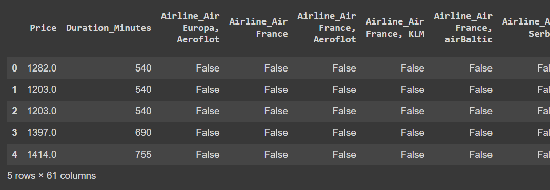
Final Dataset preview

Note: Here, we are just showcasing a part of dataset as there are a huge number of columns.

Model Training with hyperparameter tuning

Now we will train a Machine Learning model called ExtraTreesRegressor for Flight Fare prediction. Here we will define a parameter search space for Randomized Search Cross-Validation which is performed for Hyperparameter tuning. For hyperparameter tuning we will choose only useful and relevant hyperparameters which are discussed below–>

• n_estimators: It refers to the total number of trees in the forest. Having a greater number of trees can improve the model’s reliability at the expense of increased computational resources.
• max_features: t specifies the maximum number of features to evaluate when determining the optimal split.
• max_depth: It sets the limit on how deep each tree can grow. Deeper trees can capture more complex relationships but may lead to overfitting if not regularized properly.
• min_samples_split: The minimum number of samples required to split an internal node during tree construction. Higher values can prevent overfitting by ensuring nodes have enough samples.
• min_samples_leaf: It dictates the minimum number of data points that must be present at a leaf node, which aids in regulating the tree’s size and preventing overfitting by placing a limit on the number of samples per leaf.

Python3

# Defining the parameter grid for RandomizedSearchCV
param_grid = {
    'n_estimators': [100, 200, 300, 400, 500],
    'max_features': ['auto', 'sqrt', 'log2'],
    'max_depth': [None, 10, 20, 30, 40, 50],
    'min_samples_split': [2, 5, 10],
    'min_samples_leaf': [1, 2, 4]
}

# Training the ExtraTreesRegressor model with RandomizedSearchCV
etr = ExtraTreesRegressor(random_state=42)
random_search = RandomizedSearchCV(estimator=etr, param_distributions=param_grid, n_iter=100, cv=5, verbose=2, random_state=42, n_jobs=-1)
random_search.fit(X_train, y_train)

Model evaluation

Now we will evaluate our model on best hyperparameter values using various performance metrics like MAE and R2-Score.

Python3

# Getting the best estimator from the search
best_etr = random_search.best_estimator_
# Predicting on the test set
y_pred = best_etr.predict(X_test)

# Evaluating the model
mae = mean_absolute_error(y_test, y_pred)
r2 = r2_score(y_test, y_pred)

print("Best Parameters:", random_search.best_params_)
print("Mean Absolute Error (MAE):", mae)
print("R-squared Score:", r2)

Output:

Best Parameters: {'n_estimators': 200, 'min_samples_split': 2, 'min_samples_leaf': 1, 'max_features': 'log2', 'max_depth': 40}
Mean Absolute Error (MAE): 808.7640999654004
R-squared Score: 0.6479013920201813

So, we have achived a moderately well R2-Score of 65% approximately. This depicts that our model is performing well but we can get better results by using larger datasets and data transformation methods before fitting the model. Also, you can try more better models.