1. Downloading, Installing, and Starting Python SciPy
Get the Python and SciPy platform installed on your system if it is not already. One can easily follow the installation guide for it.
1.1 Install SciPy Libraries:
Working on Python version 2.7 or 3.5+.
There are 5 key libraries that you will need to install. Below is a list of the Python SciPy libraries required for this tutorial:
- scipy
- numpy
- matplotlib
- pandas
- sklearn
1.2 Start Python and Check Versions:
It is a good idea to make sure your Python environment was installed successfully and is working as expected.
The script below will help to test out the environment. It imports each library required in this tutorial and prints the version.
Type or copy and paste the following script:
Python3
import sys
print('Python: {}'.format(sys.version))
import scipy
print('scipy: {}'.format(scipy.__version__))
import numpy
print('numpy: {}'.format(numpy.__version__))
import matplotlib
print('matplotlib: {}'.format(matplotlib.__version__))
import pandas
print('pandas: {}'.format(pandas.__version__))
import sklearn
print('sklearn: {}'.format(sklearn.__version__))
|
If an error arises, stop. Now is the time to fix it.
2. Load The Data:
Dataset – Iris data
It is famous data used as the “hello world” dataset in machine learning and statistics by pretty much everyone.
The dataset contains 150 observations of iris flowers. There are four columns of measurements of the flowers in centimeters. The fifth column is the species of the flower observed. All observed flowers belong to one of three species.
2.1 Import libraries:
First, let’s import all of the modules, functions, and objects to be used.
Python3
import pandas
from pandas.plotting import scatter_matrix
import matplotlib.pyplot as plt
from sklearn import model_selection
from sklearn.metrics import classification_report
from sklearn.metrics import confusion_matrix
from sklearn.metrics import accuracy_score
from sklearn.linear_model import LogisticRegression
from sklearn.tree import DecisionTreeClassifier
from sklearn.neighbors import KNeighborsClassifier
from sklearn.discriminant_analysis import LinearDiscriminantAnalysis
from sklearn.naive_bayes import GaussianNB
from sklearn.svm import SVC
|
A working SciPy environment is required before continuing.
2.2 Load Dataset
Data can directly be loaded into the UCI Machine Learning repository.
Using pandas to load the data and exploring descriptive statistics and data visualization.
Note: The names of each column are specified when loading the data. This will help later at the time of exploring the data.
Python3
url =
names = ['sepal-length', 'sepal-width', 'petal-length',
'petal-width', 'class']
dataset = pandas.read_csv(url, names = names)
|
If you do have network problems, you can download the iris.csv file into your working directory and load it using the same method, changing the URL to the local file name.
3. Summarize the Dataset:
Now it is time to take a look at the data.
Steps to look at the data in a few different ways:
- Dimensions of the dataset.
- Peek at the data itself.
- Statistical summary of all attributes.
- Breakdown of the data by the class variable.
3.1 Dimensions of Dataset
(150, 5)
3.2 Peek at the Data
    sepal-length  sepal-width  petal-length  petal-width        class
0            5.1          3.5           1.4          0.2  Iris-setosa
1            4.9          3.0           1.4          0.2  Iris-setosa
2            4.7          3.2           1.3          0.2  Iris-setosa
3            4.6          3.1           1.5          0.2  Iris-setosa
4            5.0          3.6           1.4          0.2  Iris-setosa
5            5.4          3.9           1.7          0.4  Iris-setosa
6            4.6          3.4           1.4          0.3  Iris-setosa
7            5.0          3.4           1.5          0.2  Iris-setosa
8            4.4          2.9           1.4          0.2  Iris-setosa
9            4.9          3.1           1.5          0.1  Iris-setosa
10           5.4          3.7           1.5          0.2  Iris-setosa
11           4.8          3.4           1.6          0.2  Iris-setosa
12           4.8          3.0           1.4          0.1  Iris-setosa
13           4.3          3.0           1.1          0.1  Iris-setosa
14           5.8          4.0           1.2          0.2  Iris-setosa
15           5.7          4.4           1.5          0.4  Iris-setosa
16           5.4          3.9           1.3          0.4  Iris-setosa
17           5.1          3.5           1.4          0.3  Iris-setosa
18           5.7          3.8           1.7          0.3  Iris-setosa
19           5.1          3.8           1.5          0.3  Iris-setosa
3.3 Statistical Summary
This includes the count, mean, the min and max values as well as some percentiles.
Python3
print(dataset.describe())
|
It is clearly visible that all of the numerical values have the same scale (centimeters) and similar ranges between 0 and 8 centimeters.
       sepal-length  sepal-width  petal-length  petal-width
count    150.000000   150.000000    150.000000   150.000000
mean       5.843333     3.054000      3.758667     1.198667
std        0.828066     0.433594      1.764420     0.763161
min        4.300000     2.000000      1.000000     0.100000
25%        5.100000     2.800000      1.600000     0.300000
50%        5.800000     3.000000      4.350000     1.300000
75%        6.400000     3.300000      5.100000     1.800000
max        7.900000     4.400000      6.900000     2.500000
3.4 Class Distribution
Python3
print(dataset.groupby('class').size())
|
class
Iris-setosa        50
Iris-versicolor    50
Iris-virginica     50
4. Data Visualization
Using two types of plots:
- Univariate plots to better understand each attribute.
- Multivariate plots to better understand the relationships between attributes.
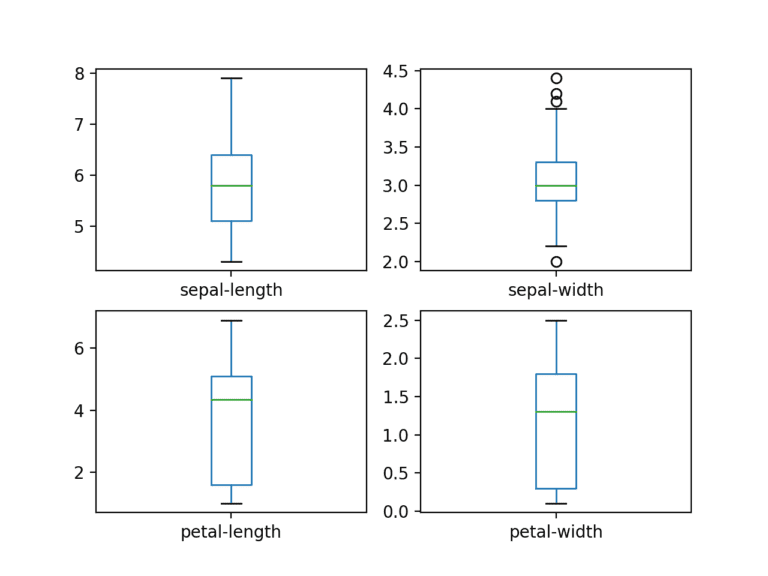
4.1 Univariate Plots
Univariate plots – plots of each individual variable.
Given that the input variables are numeric, we can create box and whisker plots of each.
Python3
dataset.plot(kind ='box', subplots = True,
layout =(2, 2), sharex = False, sharey = False)
plt.show()
|
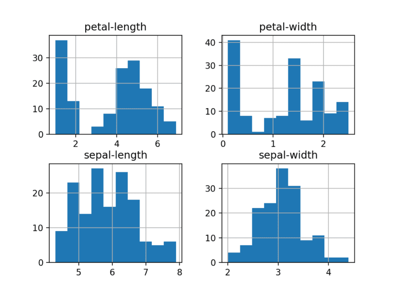
Creating a histogram of each input variable to get an idea of the distribution.
Python3
dataset.hist()
plt.show()
|
It looks like perhaps two of the input variables have a Gaussian distribution. This is useful to note as we can use algorithms that can exploit this assumption.
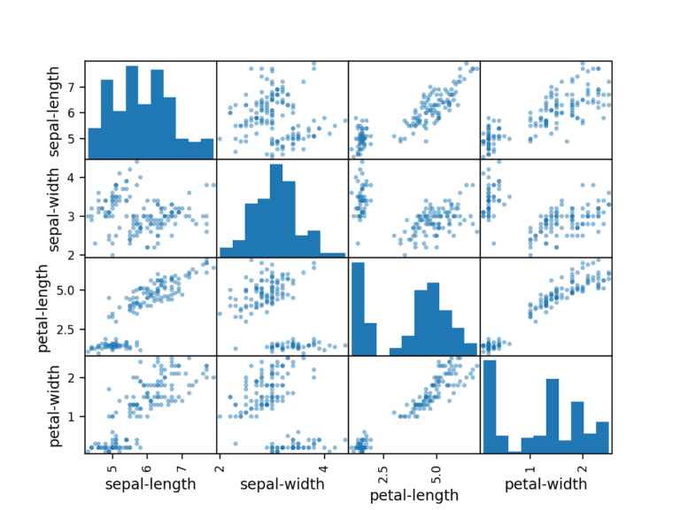
4.2 Multivariate Plots
Interactions between the variables.
First, let’s look at scatterplots of all pairs of attributes. This can be helpful to spot structured relationships between input variables.
Python3
scatter_matrix(dataset)
plt.show()
|
Note the diagonal grouping of some pairs of attributes. This suggests a high correlation and a predictable relationship.
5. Evaluate Some Algorithms
Creating some models of the data and estimate their accuracy on unseen data.
- Separate out a validation dataset.
- Set up the test harness to use 10-fold cross-validation.
- Build 5 different models to predict species from flower measurements
- Select the best model.
5.1 Create a Validation Dataset
Using statistical methods to estimate the accuracy of the models that we create on unseen data. A concrete estimate of the accuracy of the best model on unseen data is taken by evaluating it on actual unseen data.
Some data is used as testing data that the algorithms will not get to see and this data is used to get a second and independent idea of how accurate the best model might actually be.
Testing data is split into two, 80% of which we will use to train our models and 20% that we will hold back as a validation dataset.
Python3
array = dataset.values
X = array[:, 0:4]
Y = array[:, 4]
validation_size = 0.20
seed = 7
X_train, X_validation, Y_train, Y_validation = model_selection.train_test_split(
X, Y, test_size = validation_size, random_state = seed)
|
X_train and Y_train are the training data for preparing models and X_validation and Y_validation sets can be used later.
5.2 Test Harness
Using 10-fold cross-validation to estimate accuracy. This will split our dataset into 10 parts, train on 9 and test on 1 and repeat for all combinations of train-test splits.
Python3
seed = 7
scoring = 'accuracy'
|
‘Accuracy’ metric is used to evaluate models. It is the ratio of the number of correctly predicted instances divided by the total number of instances in the dataset multiplied by 100 to give a percentage (e.g. 95% accurate).
5.3 Build Models
Which algorithms would be good on this problem or what configurations to use, is not known. So, an idea is taken from the plots that some of the classes are partially linearly separable in some dimensions.
Evaluating 6 different algorithms:
- Logistic Regression (LR)
- Linear Discriminant Analysis (LDA)
- K-Nearest Neighbors (KNN).
- Classification and Regression Trees (CART).
- Gaussian Naive Bayes (NB).
- Support Vector Machines (SVM).
The algorithms chosen are a mixture of linear (LR and LDA) and nonlinear (KNN, CART, NB, and SVM) algorithms. Random number seeds are reset before each run to ensure that the evaluation of each algorithm is performed using exactly the same data splits. It ensures the results are directly comparable.
Building and evaluating the models:
Python3
models = []
models.append(('LR', LogisticRegression(solver ='liblinear', multi_class ='ovr')))
models.append(('LDA', LinearDiscriminantAnalysis()))
models.append(('KNN', KNeighborsClassifier()))
models.append(('CART', DecisionTreeClassifier()))
models.append(('NB', GaussianNB()))
models.append(('SVM', SVC(gamma ='auto')))
results = []
names = []
for name, model in models:
kfold = model_selection.KFold(n_splits = 10, random_state = seed)
cv_results = model_selection.cross_val_score(
model, X_train, Y_train, cv = kfold, scoring = scoring)
results.append(cv_results)
names.append(name)
msg = "% s: % f (% f)" % (name, cv_results.mean(), cv_results.std())
print(msg)
|
5.4 Select Best Model
Comparing the models to each other and select the most accurate. Running the example above to get the following raw results:
LR: 0.966667 (0.040825)
LDA: 0.975000 (0.038188)
KNN: 0.983333 (0.033333)
CART: 0.975000 (0.038188)
NB: 0.975000 (0.053359)
SVM: 0.991667 (0.025000)
Support Vector Machines (SVM) has the largest estimated accuracy score.
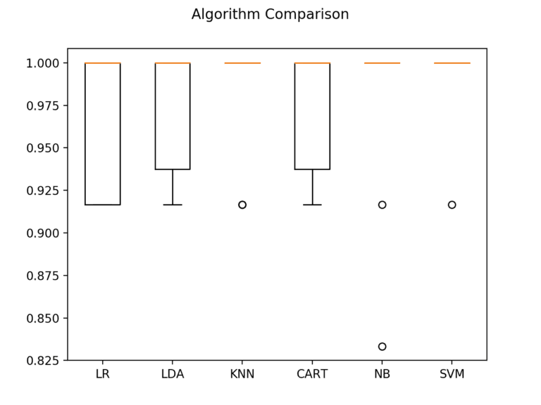
The plot of the model evaluation results is created and compares the spread and the mean accuracy of each model. There is a population of accuracy measures for each algorithm because each algorithm was evaluated 10 times (10 fold cross-validation).
Python3
fig = plt.figure()
fig.suptitle('Algorithm Comparison')
ax = fig.add_subplot(111)
plt.boxplot(results)
ax.set_xticklabels(names)
plt.show()
|
Box and whisker plots are squashed at the top of the range, with many samples achieving 100% accuracy.
6. Make Predictions
The KNN algorithm is very simple and was an accurate model based on our tests.
Running the KNN model directly on the validation set and summarizing the results as a final accuracy score, a confusion matrix, and a classification report.
Python3
knn = KNeighborsClassifier()
knn.fit(X_train, Y_train)
predictions = knn.predict(X_validation)
print(accuracy_score(Y_validation, predictions))
print(confusion_matrix(Y_validation, predictions))
print(classification_report(Y_validation, predictions))
|
Accuracy is 0.9 or 90%. The confusion matrix provides an indication of the three errors made. Finally, the classification report provides a breakdown of each class by precision, recall, f1-score, and support showing excellent results (granted the validation dataset was small).
0.9
[[ 7  0  0]
 [ 0 11  1]
 [ 0  2  9]]
                 precision    recall  f1-score   support

    Iris-setosa       1.00      1.00      1.00         7
Iris-versicolor       0.85      0.92      0.88        12
 Iris-virginica       0.90      0.82      0.86        11

      micro avg       0.90      0.90      0.90        30
      macro avg       0.92      0.91      0.91        30
   weighted avg       0.90      0.90      0.90        30
Share your thoughts in the comments
Please Login to comment...