Sklearn | Multi-dimensional Scaling (MDS) Python Implementation from Scratch

Scikit-learn (sklearn) is a Python machine-learning package that is open-source and free to use. It is Python’s most popular machine-learning library, and it is extensively used in business and academics. Scikit-learn includes a wide range of machine learning methods, including supervised learning (classification, regression), unsupervised learning (clustering, dimensionality reduction), model selection and evaluation, data preparation, and feature engineering. In this article, we will discuss an unsupervised learning technique that is commonly used to visualize the relationships between data points in a high-dimensional space by mapping them to a lower-dimensional space, such as 2D or 3D, while preserving the pairwise distances between the data points as much as possible.

Multi-dimensional Scaling (MDS)

Multi-dimensional scaling (MDS) is an unsupervised machine learning technique used to visualize the relationships between data points in a high-dimensional space by mapping them to a lower-dimensional space, such as 2D or 3D while preserving as many pairwise distances as possible.

Multi-dimensional Scaling (MDS) is a way to find similarities or differences between data points in a low-level space while keeping pairs as separate or distinct as possible. MDS is especially useful when you want to explore and discover underlying patterns or relationships in high-level data.

1. Motivation for MDS:

• MDS aims to create high-dimensional data in a low-dimensional space while preserving the spacing of data points as accurately as possible.
• Usually used in data analysis to search, reduce size and visualize data.

2. Types of MDS:

• Metric MDS: Stores the first pairs in lowercase letters away from the data points.
• Non-Metric MDS: Focuses on preserving the order of distances rather than their actual values.

3. Interpreting MDS Results:

• The x_mds data variable can be viewed to discover the structure and relationship between data points.
• MDS aims to find points in a low-dimensional space such that their connections reflect differences in high-dimensional data.
• While data points that are close to each other in the MDS chart are similar to the original data, data points that are far from each other are not similar.

Why is Multi-dimensional Scaling (MDS) important?

Multidimensional scaling (MDS) is important for many reasons, mainly because they provide a better understanding of complex data, aid in data visualization, and support decision-making in many aspects. Here is a brief summary of the main features of MDS with examples:

1. Data Simplification: MDS reduces the dimensionality of data while preserving their correlations or differences. This simplification makes it easier to interpret and visualize data, especially when dealing with high data. Example: Let’s say you have a database containing hundreds of attributes that describe various aspects of customer behaviour. By applying MDS, you can reduce these characteristics to two dimensions and create a scatter chart that presents similar groups of customers, helping you make business decisions.
2. Data Visualization: MDS creates a low-dimensional data representation that can be easily visualized. Visualization is essential for information retrieval, communication, and storytelling. Example: In geographic analysis, MDS can be used to create city plans based on remote areas, making it easier to identify differences between locations or plan transportation.

Application of MDS

• MDS is frequently used in many fields such as psychology, biology, geography and economics to perform tasks such as cluster analysis, visualization and data analysis.
• Can help identify hidden patterns, clusters or inconsistencies in data.

Advanced Multi-dimensional Scaling (MDS)

Advanced multidimensional extensions (MDS) technology is an extension or modification of the classic MDS that provides greater flexibility, functionality or enhanced functionality in certain situations. This advanced technology is designed to process complex data and provide effective solutions for a variety of applications. Here are some MDS skills:

1. Non-Metric MDS: Non-metric MDS is an extension of classical MDS that focuses on preserving the specification of variables, not the variables themselves. Useful when the variable data is not on a positive or non-linear scale. Information must be captured.
2. Kernel MDS: Kernel MDS uses kernel processing to perform MDS in a high-performance environment. Can capture non-linear relationships in data by implicitly mapping data points to higher level locations.
3. Metric Learning MDS: Metric learning MDS aims to learn the appropriate metric (distance function) while minimizing the residuals. Useful when the original measurement does not fit the data model and a custom measurement is required.

Limitations of MDS

1. The curse of dimensionality: As calculations become more complex and results become more difficult to interpret, MDS can suffer from high throughput.
2. It is very sensitive to noise. MDS is sensitive to noise and outliers in the data; This may distort the representation in low-dimensional space.
3. Non-linearity: MDS assumes a relationship between data points, but this is not true for all cases. If your data has a non-linear relationship, MDS may produce erroneous results.
4. Choose a measurement. The choice of distance measurement is important in MDS. Different measures can produce different results, and choosing the right measure can be difficult.
5. Scale uncertainty: MDS solutions suffer from scale uncertainty; This means that the same relationship can be represented in different ways, making it difficult to interpret correctly in a low place.
6. Dimensionality: Determining visual dimensions for low-dimensional space can be subjective and may require registration knowledge or other skills.
7. Computational complexity: MDS operations for large data sets can be computationally demanding and time-consuming, which can limit their effectiveness. Note: MDS often needs to store different matrices or distance matrices; this can increase memory usage for large data sets.
8. Non-Euclidean data: MDS assumes Euclidean distance, which may not work for all data types such as categorical or ordinal data.
9. Data is missing. MDS essentially discards some data when reducing the size, and low-resolution representations may not capture all the nuances of the original data.

Mathematical Formulation of MDS

The basic idea of ​​MDS is to find a general process in low-dimensional space that minimizes the variance (D) in high-dimensional space and the dependent variance (d) in low-dimensional space.

Mathematically this can be expressed as: Given a dissimilarity or distance matrix D representing the difference between points i and j in a space where Dij is higher (e.g. Euclidean distance), MDS attempts to find the set of coordinates xi and xj. This is done in a low-dimensional space such that the Euclidean distance between xi and xj (denoted by dij) is as close as possible to the difference Dij.

The target task to reduce MDS can be defined as follows:

Where:

• Wij is a weight that can be used to emphasize or de-emphasize specific distances.
• dij is the Euclidean distance between data points i and j in the lower-dimensional space.
• Dij is the dissimilarity (distance) between data points i and j in the high-dimensional space.

Why MDS is better than other dimensionality reduction methods

1. Distance: MDS clearly shows the distance or difference between data points. This is especially true when relationships between data points are important for analysis or visualization.
2. Distance measurements: MDS is versatile and can handle a variety of distance measurements, including non-Euclidean distances, making it suitable for a wide range of data. Other methods, such as SNE or autoencoders, are easier to explain. Coordinates correspond directly to data points in low-level space.
3. Solid mathematical foundation: MDS has a good mathematical foundation, making it useful and interpretable.
4. History: MDS has a long history and is widely used in fields such as psychology, geography, and social sciences, making it popular and reliable.

MDS on Digits Dataset

Dataset:

• Digital data consists of grayscale images consisting of alphanumeric characters (0 to 9), each represented as an 8×8 pixel image.
• Each image is converted into a combination of 64 elements. This means that each data point in the dataset is a vector of 64 values ​​corresponding to the pixel value in the digital image.
• It is often used in tasks such as recognizing and distributing numbers.

Python3

import numpy as np
import matplotlib.pyplot as plt
from sklearn.datasets import load_digits
from sklearn.manifold import MDS

# Load a sample dataset (e.g., the digits dataset)
data = load_digits()
X, y = data.data, data.target

print('Original Dimesnion of X = ', X.shape)
# Create an MDS model with the desired number of dimensions
# Number of dimensions for visualization
n_components = 2
mds = MDS(n_components=n_components)

# Fit the MDS model to your data
X_reduced = mds.fit_transform(X)

print('Dimesnion of X after MDS = ',X_reduced.shape)

# Visualize the reduced data
plt.figure(figsize=(8, 6))
plt.scatter(X_reduced[:, 0], X_reduced[:, 1], c=y, cmap=plt.cm.get_cmap("jet", 10))
plt.colorbar(label='Digit Label', ticks=range(10))
plt.title("MDS Visualization of Digits Dataset")
plt.xlabel("MDS Dimension 1")
plt.ylabel("MDS Dimension 2")
plt.show()

Output:

Original Dimesnion of X =  (1797, 64)

Dimesnion of X after MDS =  (1797, 2)

Dimensions of X (Original Data):

• n_samples — number of points (digital image)
• n_features is the number of features per data point (64 in this case corresponds to 64 pixels in an 8×8 image).

Dimensions After Reducing It:

• The code provided uses multidimensional scaling (MDS) to reduce the length of the data to two dimensions for visualization purposes. Therefore, the length of the reduced X_reduced data after applying MDS is (n_samples, n_components). Where:
  • n_samples equals the original data representing the data content (image of numbers).
  • The value of n_comComponents is 2. This means that the dimensions for the study were reduced to two dimensions (MDS Dimension 1 and MDS Dimension 2).

The output of this code is a scatter plot where each point represents a digit image, and the position of the points in the plot is determined by the MDS algorithm, aiming to preserve the pairwise distances between the data points as much as possible while reducing the dimensionality to 2D. The colors of the points correspond to the actual digit labels, allowing you to see how well the MDS algorithm separates the different digit classes in the reduced space.

MDS on Make_blobs dataset

Python3

import numpy as np
import matplotlib.pyplot as plt
from sklearn.datasets import make_blobs
from sklearn.manifold import MDS

# Generate a sample dataset (you can replace this with your own data)
X, _ = make_blobs(n_samples=100, n_features=3, centers=2, random_state=42)

print('Original Dimension of X : ', X.shape)
# Perform MDS to reduce the dimensionality to 2D

mds = MDS(n_components=2, random_state=42)
X_2d = mds.fit_transform(X)

print('Dimension of X after MDS : ', X_2d.shape)

# Plot the results
plt.scatter(X_2d[:, 0], X_2d[:, 1])
plt.title("MDS Visualization")
plt.xlabel("MDS Dimension 1")
plt.ylabel("MDS Dimension 2")
plt.show()

Output:

Original Dimension of X :  (100, 3)

Dimension of X after MDS :  (100, 2)

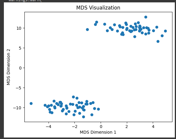
2nd code Output

• Original Dimesnion of X = (100,3)
• After applying MDS, the resulting dataset X_2d has 100 samples and 2 features (n_samples=100, n_components=2).
• This means that the data has been successfully transformed from its original 3D space to a 2D space.

The output of this code is a scatter plot displaying the 2D representation of the original dataset after applying MDS. The points in the scatter plot represent the data points in the reduced 2D space. Depending on the original data distribution and the chosen random seed, you’ll see a visualization of how the data points are positioned in a 2D space, preserving certain relationships between them.

Conclusion

In summary, multidimensional scaling (MDS) is a powerful dimensionality reduction and data visualization process that plays an important role in many fields and applications. In fact, it is a versatile and indispensable tool for multidimensional scaling, data analysis, visualization and pattern recognition. Its ability to transform complex data into meaningful and understandable content makes it a valuable tool in the interdisciplinary research toolkit of data scientists, analysts, and researchers.